Becoming Acquainted with Excel
Excel is a powerful and
versatile spreadsheet program that can be used for both business and personal needs. It has amazing
capabilities
that you can use to make any type of data you record more streamlined and productive. In the first chapter,
you�ll learn the basics of creating worksheets, and how to use the Ribbon, a feature which drives the
user-friendly resources in Excel.
After reading
and working through
this chapter you should be able to
�
Know what Excel is and know some of its capabilities
�
Create, save, and open a workbook
�
Identify the current cell
�
Use the Ribbon
�
Use and customize the Quick Access
Toolbar
�
Enter data in a worksheet
�
Get help by using ScreenTips and the
Tellmewhatyouwanttodo features
What Is Excel?
Excel is an electronic
spreadsheet program. A spreadsheet is a grid of cells organized into rows and
columns in which you enter and
store your data. Excel can meet both your personal and professional needs.
Using Excel, you can do all of the following:
�
Create, edit, sort, analyze, summarize, and format data as well as graph it.
�
Keep budgets and handle payroll
�
Track investments, loans,
sales, inventory, etc.
�
Perform What-If
Analysis to determine such things as �if the price of gas went up 20
cents per gallon� by how much would that decrease my profit, or �if I extend my loan
payments from 15 years to 20 years� by how much will that affect my monthly payments,
total payments, and total interest.
One can improve
the appearance of a spreadsheet or better convey what you want a spreadsheet to
say by adding pictures, clip art, shapes, smart art, video, and audio.
1
CHAPTER 1 ■ BECOMING ACQUAINTED WITH EXCEL
Microsoft Office
is Microsoft�s most profitable product.
Microsoft devoted most of its effort in Microsoft Office
2016 to updating
Excel. Microsoft made few changes
to its other products in Office.
History of Spreadsheets
VisiCalc (short for Visible Calculator) was the first computerized spreadsheet available to the public. It
was created by Dan Bricklin and Bob Frankston in 1979 for the Apple IIe and then released in 1981 for the
newly created IBM PC. Up to this point, sales of personal computers had been slow because there wasn�t a lot
you could do with them. Early PCs were very expensive and there weren�t any prewritten applications. They
were mostly purchased by computer programmers who thought they were fascinating and it gave them a chance to
practice programming at home. At this point, programmers worked on large-scale computers called mainframes.
At that time, you couldn�t go to a store and buy software like you can today. Back then, company programmers
wrote all the programs that the company needed themselves. Each company
wrote its own payroll
program, its own inventory program, etc. Companies didn�t share the software
with each other. With VisiCalc,
businesses now had a product that could be of great benefit. Sales of personal computers took off. VisiCalc
became
the world�s first Super App. VisiCalc also started a revolution in businesses being started for the sole
purpose of creating software to be sold to the public.
The Lotus 1-2-3
Spreadsheet program was released in 1983. It was made specifically for the IBM
PC. It was faster and had better graphics than VisiCalc and soon replaced it.
Lotus 1-2-3 greatly increased the sales of the IBM PC.
Microsoft Excel has dominated the spreadsheet market
since the 1990s.
This Book
An Excel book that taught you every possible
option would be too large
for you to carry. As you go through the
material in the book, explore
the different options
and try different things, think about
how you could
use what is being taught
in different environments. Don�t just click
here and enter
that, because that is what the book
is telling you to do without thinking
about what it is you are doing.
Excel is so powerful and is capable
of doing so many things.
Be a free thinker and think about
how you could
use Excel to solve various
problems.
Throughout this book you will be reading about an Excel topic followed by a practice. You can learn by
reading, but to fully comprehend the different topics you should do the exercises. Many illustrations are
included to make it easier to follow along and comprehend.

■
Note� Your Excel program might not match perfectly
with this workbook. Microsoft is
constantly making changes to the
program through the Internet.

Excel Navigation Basics
Before we can do anything with Excel, let�s get to know the main parts of the program. Figure 1-1 shows an
Excel workbook. The arrows have been added to highlight the purpose of the different areas of the workbook.
2
CHAPTER 1 ■ BECOMING ACQUAINTED WITH EXCEL
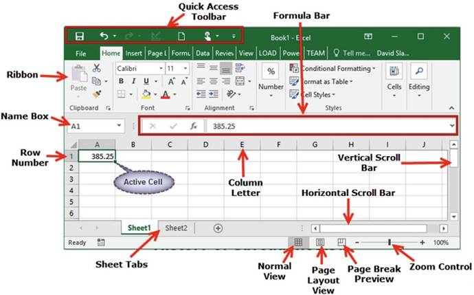
Figure 1-1. An Excel workbook
Figure 1-1 shows essential components of the workbook and worksheet. I�ll work clockwise around the sheet
starting with the Quick Access Toolbar (QAT).
�
The QAT is a shortcut
tool for storing
the commands you use most often and want quick
access to.
�
The formula bar
shows the formulas for the current selected cell. Excel displays the result
of the formulas, not the formula itself, in each cell. This bar lets you see
the formula that is producing the cell results.
�
The vertical scroll bar and horizontal scroll bar allow you to move through
the worksheet page.
�
The Zoom control,
Page Break Preview,
Page Layout View and Normal
View are buttons that allow
you to control how you are viewing
the worksheet.
�
The Zoom control
lets you increase
or decrease the size (Zoom percentage) of the worksheet on your screen.
�
Page Break Preview allows you to control where one page ends and another begins. This helps make
the worksheet more user friendly by allowing pages to be organized in a way that makes sense to the user.
�
Page Layout View shows how the page will look when it is printed.
Use this function
to ensure the printed workbook
will be neat and easy to read.
�
Normal View is the default view. It shows how the workbook looks while you are working on it.
Sheet Tabs let you select the worksheet that you want to work on or view. Many workbooks in Excel will have
multiple sheets.
3
CHAPTER 1 ■ BECOMING ACQUAINTED WITH EXCEL
The row number tells
you what row you are on in the workbook. Excel has a potential of 1,048,576 rows. Columns
are identified by letters. There
are 16,384 columns
in an Excel spreadsheet. This means that a single worksheet contains
more than 17 billion cells.
Each cell can hold 32,767
characters. How many worksheets you can have in a workbook depends
upon your computer�s available memory. Each cell is identified by an address
which consists of the column
letter and the row number.
The Name box displays
the address of the cell where you are at the moment.
The Name box in Figure
1-1 displays A1which is the
address of the current
active cell. The Ribbon provides access to all of Excel�s capabilities. The
Ribbon will be
discussed in
much greater detail later in this chapter and in subsequent chapters.
Creating, Saving, and Opening Workbooks
The first step is to create
a workbook. Next, you must make sure to save your work as you go. You should consider
what you want in the workbook and what it should be named before you create and
save it. This will make it easy to open
and use it again.
We�ll start our
Excel journey by creating a new workbook and then examine the different parts
of the workbook. How you start
Excel depends upon your operating system. Excel starts just like any other application you use.

In this exercise, we�ll create a simple blank workbook and save it.
1.
Start your Excel program. If the Excel start button is on your status bar you can click on it,
otherwise start Excel the way you normally start a program.
Figure 1-2 shows the opening
window.
4
CHAPTER 1 ■ BECOMING ACQUAINTED WITH EXCEL
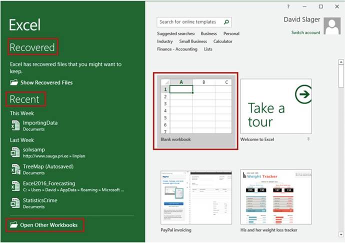
Figure 1-2. Excel starting window
5
CHAPTER 1 ■ BECOMING ACQUAINTED WITH EXCEL

■
NoteThe file names
on the left side of your window
will not be the same as those
shown in Figure
1-2 because they are the names
of the files that I have opened.
2.
When you start a new workbook, you have two choices:
�
You can start with a blank workbook by clicking the Blank workbook
button, or
�
You can click one of the many template
buttons to create
a new workbook based on the templates you selected.
Click Blank workbook for this exercise.
3.
Click any cell, type any value
you want, and then press the Enter
key.
4.
Click the Save button
 �located on the QAT at the top left of your window (see Figure 1-1). The first time you save the
workbook
Excel will display
the File tab with Save As highlighted. See Figure 1-3.
�located on the QAT at the top left of your window (see Figure 1-1). The first time you save the
workbook
Excel will display
the File tab with Save As highlighted. See Figure 1-3.
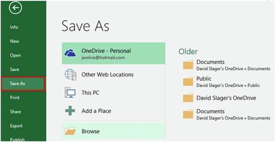
Figure1-3.Placestosaveyourworkbook

■
NoteYou will learn
a lot more about saving
workbooks from the File tab (known as the Backstage) in Chapter 6.
You can save your file to many different locations. If you are using this book in a school,
you should ask your instructor where to save your files.
The folders on the right
are places where
you have recently
saved files. Selecting one of these
locations or clicking
on the Browse button will bring up the Save As window.
5.
Click Browse.
Your Save As window may look slightly
different than the one in Figure 1-4 depending upon your version of Windows. If you have used File Explorer
before,
this window works the same
6
CHAPTER 1 ■ BECOMING ACQUAINTED WITH EXCEL
way. Click a folder and then, if need be, click a folder within
that folder as you build the path to where you want the file to be saved. The path is the drive and folders
that you must go through
to get to the file. The workbook
being saved in Figure 1-4 is set to be saved in the Documents folder.
You may want to store the file directly in the My Documents folder or you may want to create a folder under
your My Documents
folder and then store your files in
it. The File name is Book1.xlsx by default. You should change
the name to something more relevant to what you are working
on. The File name can be changed
by dragging across
the word Book1
and then typing
a new name.
6.
Create the path to where
you want your workbook saved
by clicking on the folders
in the left pane of the Save As window
until you are at the location where
you want to store your files.
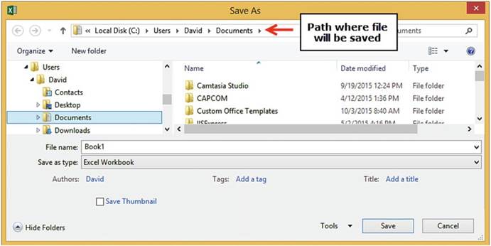
Figure 1-4. Save As window
7.
Change the File name from Book1 to MyFirstWorkbook. Excel
adds an extension of
.xlsx to the
file name. Make sure the Save as type is Excel Workbook(*.xlsx).
8.
Click the Save button.
9.
Enter any value you want in another cell then press Enter.
10.
Click the Save button
 �located on the QAT. Since you previously saved the file, the Save As window doesn�t
appear.
Excel saves the file with all the changes you made to it.
�located on the QAT. Since you previously saved the file, the Save As window doesn�t
appear.
Excel saves the file with all the changes you made to it.
11.
Close Excel by clicking the X in the upper right corner.

7
CHAPTER 1 ■ BECOMING ACQUAINTED WITH EXCEL
This exercise
showed you the basics of creating a workbook. Next,
you�ll practice opening
the same workbook
to continue working
on it.

In this exercise, we�ll open the file we created in the last exercise, make some changes, and then save with
a
new name. This will create a new
workbook.
1.
Start Excel.
The window in Figure 1-5 displays
with the MyFirstWorkbook file you created in the previous exercise listed in the Recent list.
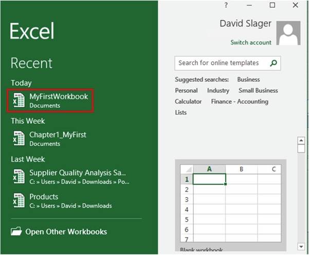
Figure1-5.Openarecentlyusedworkbook
2.
Click MyFirstWorkbook. The
workbook opens.
Next, we will add additional cell values to
this workbook and then save it under a different name.
Create
Another Workbook Under a Different Name
1.
Enter any value you want in a blank cell.
2.
Click the Ribbon�s File tab.
8
CHAPTER 1 ■ BECOMING ACQUAINTED WITH EXCEL
3.
In the left pane click
Save As.
4.
Click Browse
5.
You can save this file in the same Documents folder where
you saved MyFirstWorkbook. Change
the name to MySecondWorkbook and click the Save button.

You now have two separate workbooks; one named MyFirstWorkbook and another named MySecondWorkbook.
MySecondWorkbook contains the same data as MyFirstWork plus the additional cell value you added. Next,
you�ll learn about the Ribbon. This feature gives you access to the editing and customization options that
allow you to make Excel meet your exact needs.
Getting to Know the Ribbon
Starting with Office 2007, Microsoft Office quit using drop-down menus in favor of a tab design called the
Ribbon. See Figure 1-6
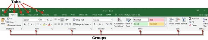
Figure1-6.IllustratestheRibbonstabsandgroups
The Ribbon consists of tabs, groups,
and command buttons.
The default Excel Ribbon contains
the following tabs: File, Home, Insert,
Page Layout, Formulas,
Data, Review, View, and PowerPivot. Your Ribbon may include
additional tabs depending
upon your setup. Each tab is broken up into groups. The buttons are organized within those groups. Office
2016 lets you alter the Ribbon to meet your own needs. You can create your own tabs or add new
groups within your tabs. You can place the commands
you use most often in your own groups.
Ribbon Contextual Tabs
In addition to the tabs
that you see when you start Excel, there are many other tabs that appear and disappear depending on what you
are
working on. These are called context-sensitivetabsbecause they are displayed based on the
contextin which you are using
them. These context-sensitive tabs will appear when you are working on such things as
charts, drawings, pictures, pivot tables and pivot charts, SmartArt graphics, header or footers, etc.
Contextual tabs have an additional label that appears above the tab. The
labels have different
background colors. Figure 1-7 shows the contextual Format tab that appears when you are working with
pictures. It has a
label of Picture Tools
above it.
Figure 1-8 shows the two additional
tabs that appear when you click
a chart in your worksheet: a Design tab, and a Format tab.
9
CHAPTER 1 ■ BECOMING ACQUAINTED WITH EXCEL
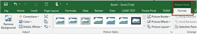
Figure 1-7.Additional tab displayed when an image
is selected
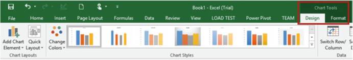
Figure 1-8.Additional tabs displayed when a chart
is selected
These additional tabs appear under a Chart Tools label. These tabs appear only as long as the object that
caused them to appear is active. Clicking off the object to something else removes the tabs.
Resizing the Ribbon
Resizing the Excel window
resizes the Ribbon. As you shrink the size of the window, the buttons start to
align vertically as shown in Figure 1-9.
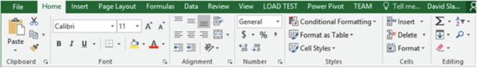
Figure1-9.Buttonsaligningvertically
Shrinking the
size of the Ribbon further as shown in Figure 1-10 makes the buttons disappear. Clicking an arrow in
the group will make that group�s buttons display below the Ribbon.
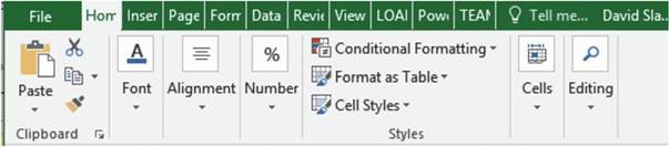
Figure1-10.ResizedRibbonmaynotshowbuttons
10
CHAPTER 1 ■ BECOMING ACQUAINTED WITH EXCEL
As you work, you may need to adjust
the size of the Ribbon
to accommodate your working space.
The next exercise
shows you how.

If you see the Restore
Down button (Figure
1-11) in the upper right-hand corner of your window that means that your window
is currently at its maximum
size. You can�t
shrink the size of the window while
your screen is maximized.

Figure 1-11. Restore Down button
1.
If the Restore Down button is displayed click it.
2.
Move your cursor to the right edge of the window. The cursor will change to a double
arrow. Drag the right edge toward the left to shrink the window. As you drag the window notice how the
buttons
start aligning vertically and as you drag farther
to the left the buttons
in the group start disappearing.
3.
Click the Maximize
button (Figure 1-12)

Figure 1-12. Maximize button
Your window should now be maximized
and the Ribbon should be displaying all of its command buttons.
Using Dialog Box Launchers
At the bottom right corner
of some Ribbon groups are boxed arrows. See Figure 1-13. They are called dialog box launchers. Dialog box
launchers
present a set of options to select from. A dialog box is a window that has options to select from, which you
must
respond to before you can return to another window. It usually has an OK button and a Cancel
button.
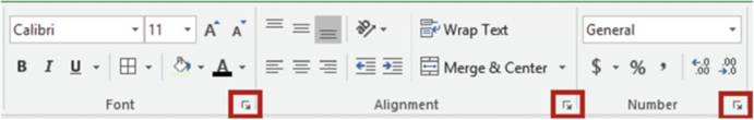
Figure 1-13. Dialog box launchers
11
CHAPTER 1 ■ BECOMING ACQUAINTED WITH EXCEL
Clicking the dialog box launcher for the Font group, Alignment group, or Number group will bring up the
Format Cells dialog box in Figure 1-14.
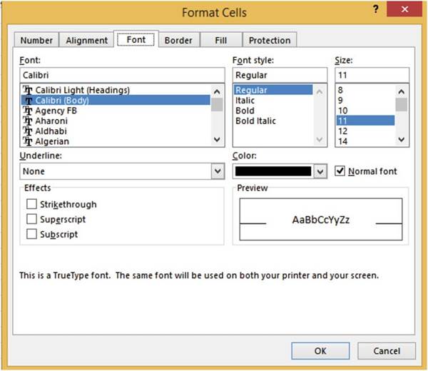
Figure1-14.FormatCellsdialogboxstartedfromtheFontdialogboxlauncher
If you click the Font group�s dialog box launcher the Font tab will be selected. If you click the Alignment
group�s dialog box launcher the Alignment tab will be selected. We will work with dialog box launchers in
later chapters.
Minimizing and Hiding the Ribbon
If you think the Ribbon is
taking up too much of your window space, you can either minimize it so that it only displays the tab names
or you can
hide it completely. Clicking the Ribbon display button in the upper right-hand corner of the Excel window
displays three options. See Figure 1-15.
12
CHAPTER 1 ■ BECOMING ACQUAINTED WITH EXCEL
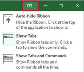
Figure 1-15. Three Ribbon options
The options are:
�
Auto-hide Ribbon: Puts your Excel workbook in full-screen mode and hides the Ribbon completely.
When your Ribbon is in Auto-hide mode you will see this
 in the top right corner of your window. Clicking the three dots or anywhere to the left of them at
the top of the screen will bring back the Ribbon. When you click inside the spreadsheet the Ribbon will
disappear again.
in the top right corner of your window. Clicking the three dots or anywhere to the left of them at
the top of the screen will bring back the Ribbon. When you click inside the spreadsheet the Ribbon will
disappear again.
�
Show Tabs: Shows
only the Ribbon tabs. Clicking a tab will display the groups with their buttons. Clicking anywhere on the
spreadsheet will hide the groups
and their buttons again. Pressing Ctrl + F1 works like a
toggle switch while in this mode by hiding and unhiding the groups and buttons.
�
Show Tabs and Commands: This options makes
the Ribbon display
in full at all times.
You
can also collapse
the Ribbon by clicking the up arrow
 �at the far right
side of the Ribbon.
�at the far right
side of the Ribbon.
Using Ribbon Shortcuts
You were always able to use
keyboard shortcuts when selecting menu items in Microsoft Office 2003 and previous versions. Microsoft kept
this
capability with the Ribbon. Pressing
the Alt key on your keyboard brings up the shortcut keys as shown in Figure 1-16 for each of the Tabs as
well as the
QAT. Keying one of the shortcut
keys for one of the Quick Access Toolbar buttons will perform that command.
Entering the shortcut key for a Ribbon tab will make that tab active. As you can see from Figure 1-16
pressing the F key will make the File tab active
and pressing the H key will make the Home tab active.
Notice
that the N key is used for the Insert tab. Most of the letters
have no relation
to the names of the options.
13
CHAPTER 1 ■ BECOMING ACQUAINTED WITH EXCEL
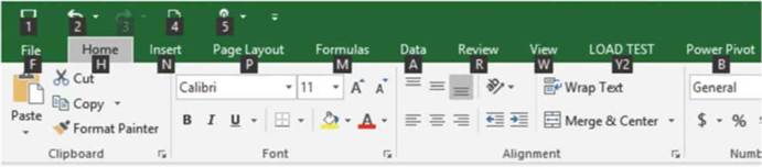
Figure 1-16.Shortcut keys for Ribbon tabs and the Quick Access Toolbar
When you press
the letter key for the tab you want to use, shortcut keys appear for every
option on that tab. Figure 1-17 shows the shortcut keys for
all the options on the Home tab. Notice, you may need to enter more than
one letter for the shortcut.
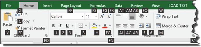
Figure1-17.ShortcutkeysforHometabcommands
Pressing a shortcut key from a tab performs that command or it will display more shortcut keys if the
command has more options available. For example, to use the keyboard to apply the Merge & Center option
you would do the following:
1.
Press the Alt key then press the H key to select the Home tab.
2.
Press Mto select the Merge button.
3.
Then press
C to select
the Merge &
Center option. See Figure 1-18.
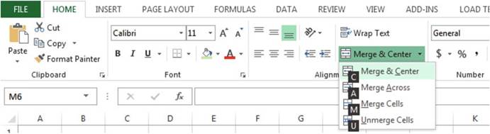
Figure 1-18.Shortcuts for commands under the Merge
& Center category
14
CHAPTER 1 ■ BECOMING ACQUAINTED WITH EXCEL

■
Note� Even if the tab is active for the command you want to use, you must still
press the Alt key and then the shortcut key for the tab.
In other words, if the
shortcut key isn�t displayed, you
can�t use it.

You should
now be able to use the Ribbon
to move around
and enter data into the worksheet. The Ribbon drives
the functionality of the Excel
program.
Besides using commands from the Ribbon
you can select
them from a QAT, which is what we�ll cover in the next section.
Quick Access Toolbar
The
Quick Access Toolbar
provides a quick and convenient place for you to store
and access
�
the tools that you use most often
�
tools that are not normally found on the
Ribbon
�
macros that you create
By default, the Quick Access Toolbar shown in Figure 1-19 is located above the Ribbon in the upper left- hand
corner of the Excel window.

Figure 1-19. Quick Access Toolbar
By default, the QAT displays
�
the save button,
which uses a diskette for an icon
�
the undo and redo buttons
�
a drop-down button from which you can select other tools to be displayed on the QAT Clicking the
drop-down button on the right side of the QAT displays the Customize Quick Access
Toolbar from which you can select
other buttons to be added
to your QAT. See Figure
1-20.
15
CHAPTER 1 ■ BECOMING ACQUAINTED WITH EXCEL
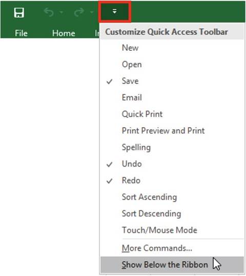
Figure 1-20.Click the drop-down button to select
Items to Add to or Remove from the QAT
The QAT can be moved below the Ribbon by selecting
the Show Below the Ribbon option from the
drop-down menu. This may be a better place for it since it will provide more room for additional tools.
Switch Between
Touch and Mouse Mode
Because many monitors today
are touch screen, Microsoft has added a Touch/Mouse Mode button. This button can be added to the QAT by
selecting it from the QAT drop-down menu. See Figure 1-20. Clicking the down arrow of the Touch/Mouse Mode
button displays the two options shown in Figure 1-21.
16
CHAPTER 1 ■ BECOMING ACQUAINTED WITH EXCEL
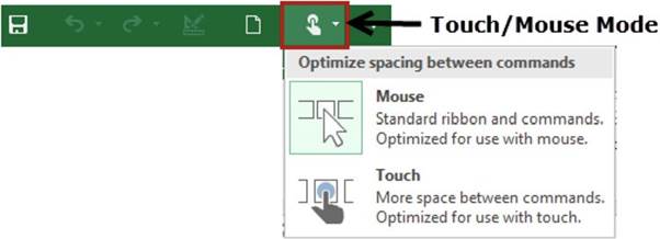
Figure1-21.OptionsforoptimizingRibbonforusingtheMouseorTouchMonitor
The Touch
option is for those users who are using touch monitors. Selecting the touch
option places
more space
between the Ribbon buttons as shown in Figure 1-22, making it easier to select the
correct button with your finger.
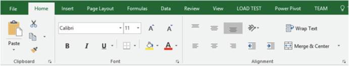
Figure1-22.RibbonsetupforTouchscreenmonitors
Changing the Touch/Mouse mode in any of the Microsoft Office
products changes it for all the office
products.
You can easily remove a button from the QAT by either right-clicking the button you wish to remove and
selecting Remove from Quick Access Toolbar or you can click the drop-down button, then click the checked
item you wish to remove.
Your QAT is not
limited to the items appearing in the Customize Quick Access Toolbar menu.
Buttons that are on the Ribbon can
be added to the QAT by right-clicking a Ribbon button and then selecting Add to Quick Access Toolbar from
the menu.
See Figure 1-23.
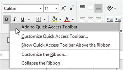
Figure1-23.AddingbuttonfromRibbontotheQAT
17
CHAPTER 1 ■ BECOMING ACQUAINTED WITH EXCEL
The order in which the buttons appear on the QAT can be rearranged. You can save your QAT customization
to a file and then later import it into another workbook.
Three
ways to get to the QAT customizations in the Excel
options window are to
�
Click the drop-down arrow on the QAT and then select
More Commands�
�
Right-click
the Ribbon and then select Customize Quick Access Toolbar�
�
Click the File tab on the Ribbon.
Select Options. Select
Quick Access Toolbar
from
the left side of the Excel
Options window.

In this exercise, you will add
command buttons to your QAT.
1.
Click the drop-down
button of the Quick Access
Toolbar and then select Print Preview
and Print from
the Customize Quick
Access Toolbar menu.
2.
Click the drop-down button of the Quick
Access Toolbar and then select
New.
3.
Click the drop-down button of the Quick
Access Toolbar and then select
Open.
The Print Preview and
Print, New, and Open buttons have
been added to the end of your Quick Access Toolbar. See Figure 1-24.

Figure 1-24. Quick Access Toolbar
Notice that the tools appear in the order
that they were selected.
4.
Right-click
the Print Preview and Print button
 �on the QAT and select Remove from Quick Access
Toolbar
�on the QAT and select Remove from Quick Access
Toolbar
5.
Right-click the QAT and then select Show Quick Access Toolbar
Below the Ribbon.
6.
Click the Review
tab on
the Ribbon. In
the Proofing
group,
right-click the Spelling
button and select Add
to Quick
Access Toolbar. Your QAT should now appear
as follows. See
Figure 1-25.

Figure 1-25. Quick Access Toolbar

18
Identifying the
Current Cell
CHAPTER 1 ■ BECOMING ACQUAINTED WITH EXCEL
Columns are represented by
letters. Rows are represented by numbers. A combination of a column letter and a row number gives each cell
a
unique address. The first cell in a worksheet would have an address of A1. A cell that is at the
intersection
of column G and row 5 would have a cell address of G5. The cell address is also called a cell reference.
Individual cells contain text, numbers, or formulas. The result of a formula is displayed in the same cell
where you
inserted the formula.
The
current (active) cell in Figure
1-26 is B6. The current cell can be identified by the following:
�
Its border is bolded.
�
Its column head and row head are highlighted.
�
The address appears in the Name Box.
�
The cell�s value or formula
is displayed in the formula
bar.
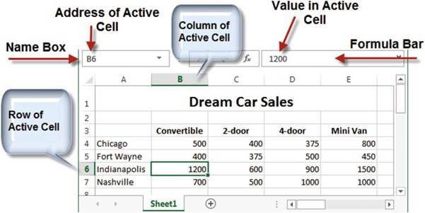
Figure1-26.Differentwaysofidentifyingthecurrentcell
Once
you�ve identified the current cell,
you are ready
to start entering
your data!
Entering Data into a Worksheet
The
data you enter
in a cell is not accepted until
you do one of the following:
�
Press the Tab key�cursor moves to the next cell
�
Press the Enter key�cursor moves to the next cell
�
Press any of the arrow
keys�cursor moves to the next cell in the direction of the arrow.
�
Click the check mark icon on the formula bar�cursor remains in the cell.
�
Pressing Ctrl + Enter�cursor remains
in the cell.
19
CHAPTER 1 ■ BECOMING ACQUAINTED WITH EXCEL

■
Note� You can�t format the data in a cell until the data has been accepted.
If you want to overwrite all the data in a cell you can click
the cell and type the new data.
If you only want to change part of the data in a cell you need to be in Edit mode. Double-clicking a cell
puts it in Edit mode;
pressing F2 will do the same. As you are typing data in a cell, the data appears
in both the active cell and
the formula bar. Because the data appears
in both the cell and the formula
bar, making changes
in either location will update the cell data.

In this exercise, you will
enter data in cells and use different options for accepting the entries.
1.
First, enter some column
headings and use the Tab key to
accept them:
a.
Type Assets in cell A1. Notice that as you�re typing
the text in cell A1 it is also being typed into the formula
bar. Press the Tab key.
b.
Type Cash in cell B1. Press the Tab key.
c.
Type Supply in cell C1. Press the Tab key.
d.
Type Land in cell D1. Press
the Enter key. Cell A2 becomes Active,
2.
Next, type Liability in
cell A2 but don�t press the Tab key. Move your cursor
over the check mark in the formula
bar. If the data in the cell hasn�t been accepted, it will change
color. See Figure
1-27. Click the Enter button
(the check mark).
The data is accepted and the button
becomes grayed out. See Figure
1-28.
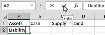
Figure1-27.ClicktheEnterbuttontoacceptthedata
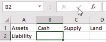
Figure 1-28.Once the data is accepted the button
becomes grayed out
20
CHAPTER 1 ■ BECOMING ACQUAINTED WITH EXCEL
3.
Press the Tab key.
4.
Type Loan in cell B2 but don�t press
the Tab key. Click the Cancel button
 �on
�on
the formula bar. The entry is cleared. Type Loan in cell B2 again.
Press Ctrl + Enter. Cell B2 remains
the active cell.
The cursor is still in cell B2 but you can�t see it.

■
Note� Another way to cancel the text you are entering
or to clear it even after it has been accepted is to move your cursor
over the square
at the bottom right of the cell (see the cell on the left).
The cursor will change to cross-hairs. Drag the cursor
toward the center
of the cell. The text will fade,
as in the cell on the right,
and
when you let go of the mouse button the text will be gone.
5.
Press the Tab key. Notice
the word Ready in
the bottom left corner of the status
bar. This means
that the cell is ready
for you to enter data into.
■
Note� If you don�t see the word Ready, then
right-click Excel�s Status bar at the bottom of the window and select Cell Mode.
6.
Type Wages into cell C2. When you start typing text in the cell the word Ready on the
status bar changes to Enter.
Press the Tab key.
7.
Double-click
inside cell C1. Looking at the
bottom left side of the status bar you should see that you are in Editmode. Change
Supply to Supplies. It doesn�t matter if you make the change in cell C1 or in the formula bar. Press Enter
when you are done.
8.
Click inside cell A2. Press
the F2 key. This is another way of placing
the cell in Edit mode. Change Liability to Liabilities. Press
Ctrl + Enter.
9.
Click once inside cell D1. Since you didn�t
double-click you are not in Edit mode. The status bar still shows Ready. Notice that the cursor
does not display. Type
the letter R. The word Land is cleared
from the cell.
Finish
typing the word Replace. Press Ctrl + Enter.
10.
Type Use in cell C5. Press the down arrow key.
11.
Type thein cell C6. Press the left arrow key.
12.
Type arrow in cell B6. Press
the up arrow key.
13.
Type keys in cell B5. Press the
right arrow key.
Getting Help
Excel provides help to the
user within the program. Screen Tips and the Tell me what you want to do
features answer questions about
formatting and entering data into your worksheet while you are working on it.
SmartLookupenables you to search on cell contents.
21
CHAPTER 1 ■ BECOMING ACQUAINTED WITH EXCEL
Screen Tips
Screen tips are a quick way of getting snippets of information about the commands on the Ribbon and some
other objects on the screen. Screen tips can be viewed by merely moving your cursor over an object. The
screen tip shows the name of the object and what it does. Some of the screen tips also provide graphic
illustrations to illustrate what the command does. Figure 1-29 shows a screen tip for the Merge & Center
button which is located on the Home tab in the Alignment group. If you wanted additional information you
could click the Tell me more link.
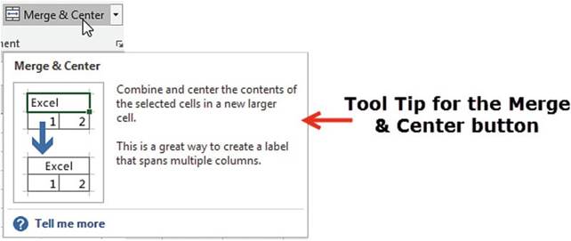
Figure1-29.ScreentipfortheMerge&Centerbutton
Excel�s Tell Me What You Want to Do Feature
This is a new feature for Office 2016;
you will also find it in Word and PowerPoint. It is located
in the tab area of the Ribbon.
When you click
the text box it displays
your most recent
requests. You can select one of the requests or you
can start typing
into the text box. Excel
displays what is available for the characters you have entered
so far.
Let�s say that I want help creating a chart. I start by entering a C into the text box. You are probably
thinking why did the list in Figure 1-30 display items that don�t all start with a C. The reason is that
Math & Trig,
More, and Financial
are groups of formulas, some of which start with a C. New from Template appears because some templates start
with a C. I can refine what appears
in the list by entering
more text.
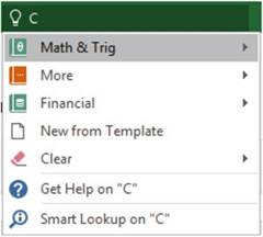
Figure 1-30.Suggested choices for Tell me what you want to do feature
22
CHAPTER 1 ■ BECOMING ACQUAINTED WITH EXCEL
After I have finished
entering the word Chart, the list has changed to items about
charts. See Figure
1-31. If a range of data was already selected,
as shown in Figure 1-32 when I clicked Create Chart in Figure 1-31,
then an Insert Chart window as shown in Figure 1-33 would display from which I could pick the chart I wanted.
If I didn�t have any data selected when I clicked
Create Chart, then I would
get a message saying how to create
a chart.
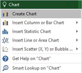
Figure
1-31.Provided suggestions after
entering the word Chart for Tell me what you want to do feature
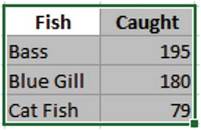
Figure 1-32.Data
selected before entering
the word Chart for Tell me what you want to do feature
23
CHAPTER 1 ■ BECOMING ACQUAINTED WITH EXCEL
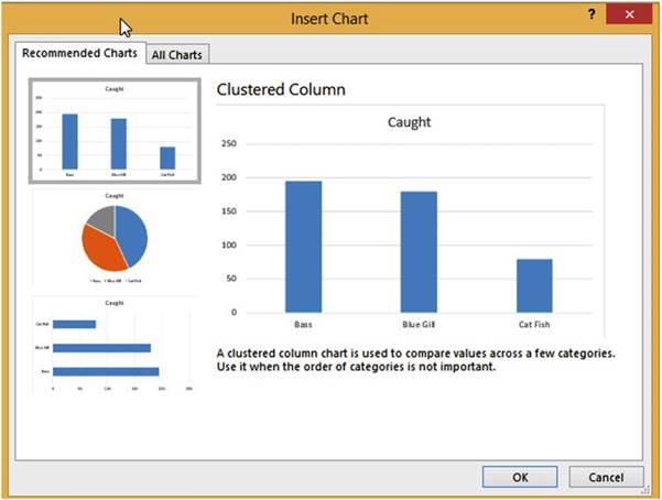
Figure 1-33. Insert Chart window
The last item
in the list in Figure 1-31 is
Smart Lookup on �Chart.� Smart Lookup is another new Office 2016 feature. Clicking Smart Lookup
performs an Internet search for what you have entered in the text box.
Smart Lookup
can also be used to do a search for text you have entered into a cell.
Right-click the cell and
select Smart Lookup. Figure 1-34 shows the results of having selected Smart Lookup from a
cell that contained the text mammoth. There are two tabs: Explore, which it shows by
default, and Define. Clicking Define, gives you the origin of the word and its
various meanings as shown in Figure 1-35.
24
CHAPTER 1 ■ BECOMING ACQUAINTED WITH EXCEL

Figure1-34.ResultofusingSmartLookupforthewordMammoth
25
CHAPTER 1 ■ BECOMING ACQUAINTED WITH EXCEL

Figure1-35.OriginofthewordMammothanditsvariousmeanings
Screen Tips and the Tell me what you want to do features
are two of the most convenient help features in Excel. You get intuitive
help answering your questions about formatting and entering data into your worksheet
while you are working on it. Smart Lookup lets you use Internet resources
without leaving your worksheet.
Summary
You�ve learned how to
create, save, and open a worksheet and how to use the Ribbon. You�ve practiced customizing the Ribbon and
creating a
Quick Access Toolbar to meet your specific needs. These are the basic skills you need to begin
utilizing the powerful features in Excel. In Chapter 2, you will practice moving around the worksheet.
You�ll learn
useful shortcuts to help you move efficiently and easily around the worksheet, reducing the time you spend
on repetitive tasks.
26
CHAPTER
2
Navigating
and Working with Worksheets
In this chapter, you�ll
learn how
to navigate
the worksheet
using the
mouse and
keyboard commands. You�ll also
become familiar with shortcuts that
help you
move quickly
between cells and begin practicing
working with multiple worksheets
within the same workbook.
After reading
and working through
this chapter you�ll be able to
�
Move between cells using the keyboard
�
Select cells
�
Work with worksheets
�
Move between worksheets
Excel is
designed for the beginner to learn and use very quickly. The exercises guide
you as you discover how to
create, enter, and manipulate data using basic functions. Remember, you build
each worksheet cell by
cell to meet your needs. It is easy to make changes as you become familiar with
Excel�s features.
Moving Between Cells Using the Keyboard
Because there are so many
cells, you need a quick way to move around the worksheet. Knowing your movement keys saves time by getting
to
the desired cell in the shortest amount of time. Click a cell to make it active or use one of the key
combinations in Table 2-1 to
jump to a particular cell.
27
CHAPTER 2 ■ NAVIGATING AND WORKING WITH WORKSHEETS
Table2-1.ShortcutMovementKeystoJumptoCells

To change the active cell��������� Press

Down to the
next cell�������� Enter
Up to the
next cell��������� Shift + Enter
Next cell��������������� Tab
Previous cell������������ Shift + Tab
First cell in the row��������� Home
Next
cell in the direction of the arrow���
Up, down, left, or right arrow keys Last cell in worksheet that contains data��
Ctrl + End
First cell in worksheet�������� Ctrl + Home
Cell in next
screen��������� Page Down
Cell in previous screen������� Page Up


This exercise will introduce you to the basic techniques for moving around
using the keyboard.
1.
Start your Excel
program.
2.
Select File ➤ New, and then select Blank workbook.
3.
Enter the data on the Sheet1 tab as shown in Figure 2-1.
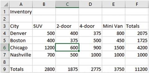
Figure2-1.Enterthesevaluesintotheworksheet
4.
Click the Save button
 �on the Quick
Access Toolbar. Since you haven�t
previously saved this file, the Save As window displays.
�on the Quick
Access Toolbar. Since you haven�t
previously saved this file, the Save As window displays.
28
CHAPTER 2 ■ NAVIGATING AND WORKING WITH WORKSHEETS
You can save the file in OneDrive
which is a
free storage location that Microsoft provides on the Web. The benefit of saving
your workbook to OneDrive
is that you can access the workbook anywhere in the
world as long
as you have access to the Internet. Another benefit is that
you can allow other
people access to it without having to e-mail it to them. If you give others
permission, they
can make changes to the workbook or enter comments in the workbook.
5.
Click This PC. Excel
displays locations you have used
most recently
as shown
in Figure
2-2.
Click Documents, which
should be displayed because you
used it
in Chapter
1.
Excel opens the Save As
dialog box.
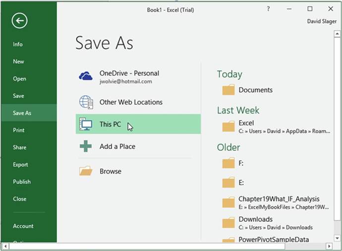
Figure2-2.TheFiletab,alsocalledBackstage
6.
Enter Chapter 2 in the File Name text box of the Save As window and click the
Save button.
Use the
Tab key
Pressing the Tab key moves the cursor one cell to the
right of the current cell.
1.
Click cell C6.
2.
Press the Tab key to move to cell D6.
3.
Press the Tab key to move to cell E6.
29
CHAPTER 2 ■ NAVIGATING AND WORKING WITH WORKSHEETS
Use the
Shift+ Tab key
Holding down
the Shift key while pressing the Tab
key moves the cursor one cell to the left.
1.
Hold down the Shift key while you press the Tab key to move to cell D6
2.
Hold down the Shift key while you press the Tab key to move to cell C6
3.
Hold down the Shift key while you press the Tab key to move to cell B6
Use the
Arrow keys
Use Arrow keys to Move to the next cell in
the direction of the arrow key
1.
Click the up arrow key to move to cell B5.
2.
Click the right arrow key to move to cell C5.
3.
Click the down arrow key to move to cell C6.
4.
Click the left arrow key to move to cell B6.
Ctrl +
End Key
Holding down the Ctrl key while pressing the End key will move the cursor to the last cell that contains
data.
1.
Hold down the Ctrl Key and Press the End key to go to cell F9.
Ctrl +
Home Key
Holding down
the Ctrl Key while pressing the Home Key will always move the cursor to Cell A1.
1.
Hold down the Ctrl Key and press the Home Key to go to cell A1.
PageDown
Key
Pressing the
PageDown Key moves the cursor down one screen
1.
Press the PageDown key twice to go down two screens.
PageUp
Key
Pressing the
PageUp key moves the cursor up one screen.
2.
Press the PageUp key twice to go up two screens.
3.
Click the Save button
 �on the Quick Access Toolbar.
In this section, you�ve learned to use the keyboard to move between cells while entering data. Next,
you�ll learn how to select cells, first by using a Mouse and then by using a keyboard.
Selecting Cells
There are several ways to
select individual cells, a range of cells, a combination of individual cells
and cell ranges, and even cells that
are nonadjacent to each other. Selecting multiple cells is useful for applying formatting to multiple cells
at the
same time or when creating formulas or deleting or inserting a complete row or column.
30
CHAPTER 2 ■ NAVIGATING AND WORKING WITH WORKSHEETS
While you are
dragging across a block of adjacent cells (see Figure 2-3), Excel displays in the Name Box how many
rows and columns are in that block. The Name Box in Figure 2-3 shows that the block of
cells spans 3 rows and 2 columns.
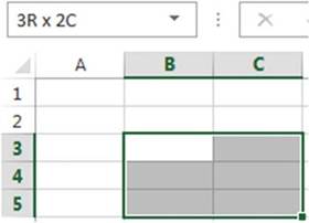
Figure2-3.Threerowsandtwocolumns
Selecting Cells Using a Mouse
Table
2-2 tells how to select different worksheet ranges using
a mouse.
Table 2-2.How
to Select Different Worksheet Ranges Using
a Mouse

To select
this����� Do this

Column����� Position the cell pointer on the column header (a letter) and then click the left mouse
button.
Row������� Position the cell pointer on the row header (a number) and then click the left mouse button.
Adjacent cells���� Drag with mouse
to select the cells in the range�or,
Click the first cell of the range, hold down the Shift key, and click the last cell in the range.

Nonadjacent cells�� Hold down the Ctrl Key while clicking
a column header,
row header, or specific cells.
All cells
in worksheet� Click the Select
All button
 .
.

In this
exercise, you select different
ranges of cells. Although we�ll
cover formatting in detail later, you can get an idea of how to use them in
this simple exercise.
Selecting
Entire Rows or Columns
1.
Open the workbook named Chapter 2, which you created in the previous
exercise.
2.
Position your cursor
on column header
B. You will see a down arrow;
hold down the left mouse button and drag across
column head C so that columns B and C are both selected. As you are dragging, you will see a box that
displays
the number of rows and columns that are currently selected. See Figure
2-4.
31
CHAPTER 2 ■ NAVIGATING AND WORKING WITH WORKSHEETS
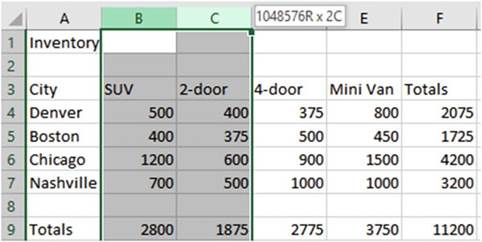
Figure 2-4.When
selecting columns heads,
Excel displays the number of rows and columns selected
3.
Click in a blank area on the worksheet to clear the selection.
4.
Position the cell pointer on row header
4. You will see a right facing arrow, hold down the left mouse button and drag down so that row headers
4, 5, 6, and 7 are selected.
As you are dragging, you will see a box that displays
the number of rows and columns that are currently
selected. See Figure
2-5.
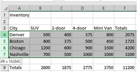
Figure 2-5.When
selecting row heads,
Excel displays the number of rows and columns selected
Selecting
Adjacent Cells
1.
Click inside cell A3 then drag to the right through cell F3.
2.
On the Ribbon�s Home tab,
in the Font group, click the
B (this will bold the selected cells).
■
Note� You can also select adjacent
cells by clicking
the cell that you want to be in the upper left cell of the range and then hold down the Shift
key while clicking
the cell you want to be the bottom right
cell of the range.

32
CHAPTER 2 ■ NAVIGATING AND WORKING WITH WORKSHEETS
3.
Click inside cell B4 hold down the Shift key and click inside cell F9
4.
On the Ribbon�s
Home tab, in the Number
group click the $ (this
will add dollar
signs, commas, and decimals to the selected
cells).
Selecting
Nonadjacent Cells
1.
Click a cell that is not part of the selection to clear the previous
selection
2.
Click Column Head C. Make
the following selections while holding the Ctrl key down:
a.
Drag across Row Heads 3 and 4
b.
Click cell E6
c.
Click cell F9
d.
Click cell A1
3.
Choose a format for the selection such as changing the font
color or changing the font size.
Selecting
all the Cells in the worksheet
1.
Click the Select All
button
 �at the top left corner of the worksheet. It is above the row heads and to the left of the column
heads.
�at the top left corner of the worksheet. It is above the row heads and to the left of the column
heads.
2.
Click the Save button on the Quick Access Toolbar.
Now that you
have learned how to select cells using a mouse, the next step is to learn how
to select cells using combinations of keys on the keyboard. The next
section has a chart detailing how to do
this.
Selecting Cells Using
a Keyboard
Table
2-3 tells how to select different worksheet ranges using
the keyboard.
Table 2-3.How to Select Workseet Ranges Using a Keyboard

To
select��������������������� Press
An entire column������������� Ctrl + spacebar
Multiple columns����������� Shift + left or right arrow
key then Ctrl
+ spacebar
An entire row��������������� Shift + spacebar
Multiple rows������������� Shift + up or down arrow
key then Shift
+ spacebar
Cells in direction of arrow key������� Shift + arrow key Cells from
current cell to beginning of the row�� Shift + Home
Go to beginning of worksheet������� Shift + Ctrl + Home Go to last
cell in worksheet containing data��� Shift + Ctrl + End
Entire worksheet������������ Ctrl + A or Ctrl + Shift + spacebar
33
CHAPTER 2 ■ NAVIGATING AND WORKING WITH WORKSHEETS
■
Note� Ctrl+A and Ctrl+Shift+spacebar select the entire worksheet if you select a
blank cell or a cell that
doesn�t have an adjacent cell containing data. If you use one of these key combinations with a cell selected
that does
have adjacent cells with data, it selects
the block of adjacent cells with data. Don�t worry if this isn�t clear. We�ll try both in the following
exercises, and you�ll see how they work.

Continue using the same workbook from the previous practice.
Selecting
an Entire Column
Pressing
Ctrl + spacebar selects all the cells in the column of the active cell.
1.
Click in cell D3.
2.
Hold down the Ctrl key and press the spacebar.
Selecting
an Entire Row
Pressing
Shift + spacebar selects all the cells in the row of the active cell.
1.
Click inside cell C3.
2.
Hold down the Shift key and press the spacebar.
Notice that the B in the Font group on the Ribbon
is highlighted. This is because
you previously bolded
this row. Click the B again. This turns off the bolding
for the row.
Selecting
Multiple Columns
1.
Move your cursor
to cell D1.
2.
Hold down the Shift key while you press the right arrow key
twice. This will select cells D1, E1, and
F1.
3.
Next hold down
Ctrl key while you press the space bar. This
will select all of columns D, E, and
F
Selecting
Multiple Rows
1.
Click cell A1.
2.
Hold down the Shift key and press the down arrow twice.
3.
Hold down the Shift key and press the space bar. This selects rows 1, 2, and 3.
Selecting
an Area
In this
exercise, you select several
different ranges using different key combinations:
1.
Click cell A1. Hold down the Shift key and keep pressing
the down arrow key until you are down to row 7. Hold down the Shift key and keep pressing
the right arrow key until you have selected columns
A to G. Hold down the Shift key and press the left arrow to deselect
column G. This selects the range A1-F7.
34
CHAPTER 2 ■ NAVIGATING AND WORKING WITH WORKSHEETS
2.
Click cell F3. Hold
down the Shift key plus the Home key. This
selects all cells from the current cell to the beginning of the row.
3.
Click cell F4. Hold
down the Shift key plus the Ctrl key plus the Home key. This selects everything from the current
cell to cell A1.
Selecting
from the Current Cell to the Last Cell Containing Data
1.
Enter 380 in cell J23. Press
Ctrl + Home to go to cell A1
2.
Press Shift + Ctrl + End. This
selects all cells between A1 and J23.
Selecting
an Entire Worksheet or All Cells
1.
Click any blank cell.
2.
Press Ctrl + A. This selects
all the cells in the worksheet.
3.
Click a blank cell again and press Shift+Ctrl+spacebar for the same
result.
Selecting
an Entire Block
1.
Click cell B5. Press Ctrl + A. This
selects all the cells in the block.
2.
Click cell B5. Press Shift+Ctrl+spacebar.
3.
Click the Save button on the Quick Access Toolbar.

You have learned how to select cells using a mouse and keyboard. Next, you�ll be learning how to select
cells by entering their cell addresses.
Select Cells by Using Their
Cell References in the Name Box
Referencing a value in a
cell by using its address is called a cell reference. A reference can be used
to identify a single cell or a range of
cells on the current worksheet or on another worksheet. You can even reference cells in other workbooks. A
reference
to cells in another workbook is called a link.
When
referencing a range of adjacent cells, the upper left cell address is listed
first, followed by a colon, and then the lower right cell�s address. The address B3:D5 includes cells
B3, C3, D3, B4, C4, D4, B5, C5, and D5. See Figure 2-6.
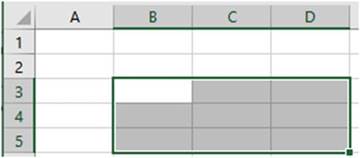
Figure2-6.TheselectedrangeisB3:D5
In Table 2-4 the first column specifies the cells to reference and the second column gives an example
of how to select that reference.
35
CHAPTER 2 ■ NAVIGATING AND WORKING WITH WORKSHEETS
Table2-4.CellSelectionExamples


Reference
to Cell(s)������������ Example
Reference a single cell. Enter column letter
followed by the row number
C12
A range of cells in a single column����
A1:A15(column A rows 1 through 15) A range of cells in a single row������ A12:E12(row 12 columns A through
E)
A range of cells in multiple rows and columns A1:F15(rows 1 through 15 in columns
A through F All cells in row 8���������� 8:8
All
cells in rows 8 through
12������ 8:12
All cells in column C���������� C:C
All cells in columns C through F����� C:F

Cell B3 on the worksheet
named Sheet1�� Sheet1!B3
The cell references can be entered into the Name Box to select those cells. You can enter any combination of
cell references that are separated by commas in the Name Box then press Enter to select those cells. Figure
2-7 shows the result of having pressed Enter after typing A2, B3:C5,E4:G5 in the Name Box. (Note that the
first cell in the last range becomes the active cell.)
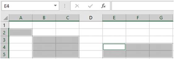
Figure 2-7.Enter
the cell addresses you wanted selected
in the Name box

The previous practices
have covered selecting cells using your mouse and your keyboard. In this exercise
you will practice
selecting individual cells,
ranges of cells,
and rows and columns of cells by entering cell addresses in the Name Box.
1.
Create a new worksheet in your Chapter 2 workbook.
2.
Enter C12 in the Name Box and then press Enter. Cell C12 should be selected.
3.
Enter A1:A15 in the Name Box and
then press Enter.
4.
Enter the other cell addresses in the Example column in Table 2-4.
5.
Enter A5, A8, B3:B7, and D4:F8 in
the Name Box then press
Enter.
36
CHAPTER 2 ■ NAVIGATING AND WORKING WITH WORKSHEETS
■
Note� If you are entering data in a selected range,
the active cell stays within that range when you press the Enter key or the Tab key.
6.
Enter A8:C10 in the Name Box
and then press Enter.
7.
It
is usually better to enter data across in rows because you can tab across to the
next cell. When you get to the last cell, press Enter to go to the
next row automatically. If you prefer to enter data going down one column and then to the next column, you
can select a range of cells
and press the Enter key after each cell entry.
a.
Type car in cell A8. Press
the Enter key.
b.
Type van. Press the Enter key.
c.
Type truck. Press the Enter key.
d.
Type semi. Press the Enter key.
e.
Type bus. Press the Enter key.
f.
Type bike. Press the Enter key.
g.
Type trike. Press the Enter key.
h.
Type train. Press the Enter key.
i.
Type skates. Press the Enter key. You now are back at cell A8.
8.
Reenter the data you entered
in each step except this time press
the Tab key after each entry.
In this section
you learned how to select cells using their cell reference. Next, you�ll be
learning to use the GoTofeature to move rapidly to
individual cells. This function becomes increasingly important when worksheets become very large over
time. When your worksheet contains extensive data, you have to be able to make quick jumps to work
efficiently.
Going Directly to Any Cell
Excel provides two methods for jumping directly to any cell. One way is to type the cell address into the
Name box and press Enter. Another way is to use the Go To feature.
Entering the
cell address in the Name box is the quicker method, but the Go To feature has
the benefit in that it stores the cells
that you jumped to previously making it easy to jump back and forth between
cells.
The Go To feature
can be accessed by clicking
the Home tab and then, in the Editing group, click the Find & Select arrow to see the drop-down menu.
See Figure 2-8. The shortcut
for this feature
is pressing Ctrl + G.
37
CHAPTER 2 ■ NAVIGATING AND WORKING WITH WORKSHEETS
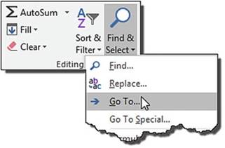
Figure2-8.SelectGoTofromtheFind&Selectbutton
Selecting the Go To� option brings
up the Go To dialog
box. See Figure
2-9.
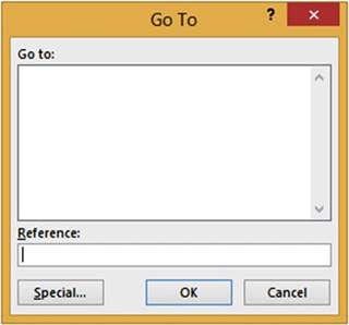
Figure 2-9. Go To dialog
box
To jump to a particular cell, you would
type the cell address for the cell you want to go to in the Reference area, and then press
Enter or Click
the OK button. Next, you learn how to work with worksheets. You will learn how to select them, rearrange
them, and change
their tab colors�as well as adding,
deleting, and hiding
them.
Worksheets
Spreadsheets in Excel are
referred to as worksheets. Individual
worksheets are stored together in a workbook. When you
save your work in Excel you do not save individual worksheets; rather, you save
the workbook.
Data entered in one worksheet can be entered into other worksheets at the same time. Data can be passed
between worksheets. Data can also be imported into worksheets from other workbooks or other sources.
A workbook can
consist of one or more worksheets. The tabs for these worksheets appear at the
bottom left-hand corner of the
screen. Clicking a sheet tab makes that sheet the current worksheet. The
current tab can be easily identified
because its tab text is bolded and has a thick line below the text.
38
CHAPTER 2 ■ NAVIGATING AND WORKING WITH WORKSHEETS

Figure 2-10. Worksheet tabs
In addition to adding and formatting data, following are some of the ways to manipulate worksheets:
�
Rename them
�
Add or Remove
them
�
Hide and Unhide
them
�
Reorder them
�
Copy them to the same workbook
�
Copy or Move them to another workbook
Naming Worksheets
If you add a second
worksheet it would be named Sheet2 by default. If you add a third worksheet it
would be named Sheet3 by default,
and so on. These names are not helpful because they don�t provide any clue as
to what is on the worksheet,
but fortunately you can rename them to something more meaningful.
There
are two ways to rename
a worksheet:
�
Right-click a sheet
tab and select Rename. This will highlight the tab you right- clicked
(see Figure 2-11a) and put the tab text in edit mode in which
you can type over the current text.(see Figure 2-11b).
�
Double-clicking a sheet tab will also put the tab text in edit mode.


Figure2-11.a)ThetabnameisinEditmode,andb)thetabhasbeenrenamed
Adding and Removing Worksheets
You can add new worksheets to your workbooks or remove them.
Worksheets can be added by doing one of the following.
�
Clicking the New Sheet button
 �. Clicking
the New Sheet button adds the new worksheet after
the currently selected
worksheet.
�. Clicking
the New Sheet button adds the new worksheet after
the currently selected
worksheet.
�
Right-click a worksheet tab and select
Insert, which displays the Insert dialog box (see Figure 2-12). Select Worksheet and click OK to add a
blank worksheet.
39
CHAPTER 2 ■ NAVIGATING AND WORKING WITH WORKSHEETS
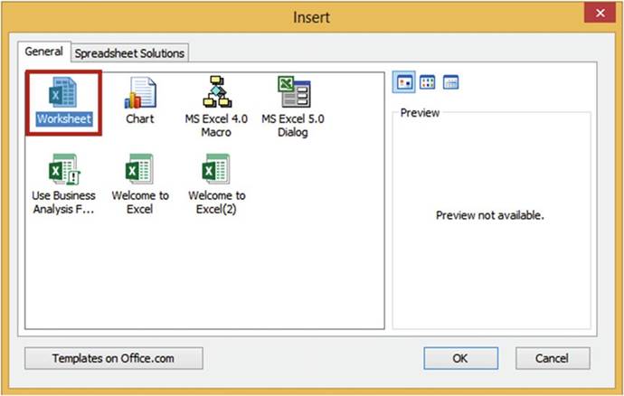
Figure 2-12.Select
Worksheet from the Insert dialog box to add a blank worksheet
You also can
use add a prebuilt worksheet known as a template. Click Spreadsheet Solutions
to see the available templates (see
Figure 2-13). There are some very nice
templates available on the Spreadsheets Solution tab. There is a Blood
Pressure Tracker, a Personal Monthly Budget template, a Loan Amortization template, and so on. Click a
template
to view it in the Preview area. Double-clicking one of these templates adds it as a worksheet in your
workbook.
40
CHAPTER 2 ■ NAVIGATING AND WORKING WITH WORKSHEETS
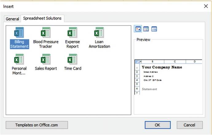
Figure 2-13. Available templates
A worksheet can be removed
by right-clicking its tab and selecting Delete.
Changing a Worksheet Tab Color
You can make
the different tabs easily distinguishable by making them different colors. You
can change the background color of each tab by right-clicking a
tab, selecting Tab Color, and then selecting a color. See Figure 2-14.
41
CHAPTER 2 ■ NAVIGATING AND WORKING WITH WORKSHEETS
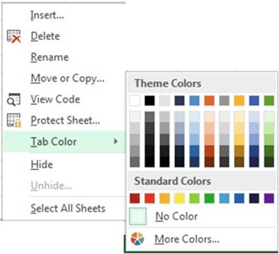
Figure2-14.Selectaworksheettabcolor
Selecting
Multiple Worksheets
You can select multiple
worksheets by holding the down Ctrl key while you click the worksheet tabs. You can select multiple
adjacent worksheets by clicking the first worksheet tab you want to use and
then holding
down the Shift
key and clicking the last worksheet tab you want to use.
Hiding and
Unhiding Worksheets
You can hide a
worksheet by right-clicking its tab and selecting Hide from the menu. Hiding
doesn�t delete
the worksheet
or change it in any way. You can bring back any worksheets you have hidden by
right-clicking
any of the
worksheet tabs and selecting Unhide� The Unhide dialog box displays all of the
worksheets you
have hidden.
To Unhide a worksheet just select the worksheet you want to redisplay and click
the OK button.
See Figure 2-15.
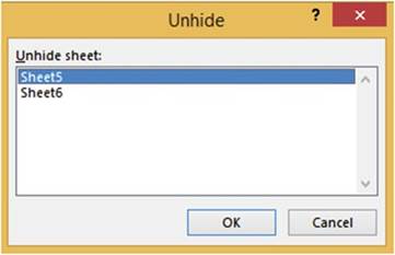
Figure2-15.SelectworksheetstoUnhide
42
CHAPTER 2 ■ NAVIGATING AND WORKING WITH WORKSHEETS
Reordering and Copying Worksheets
You can change the order of
the worksheets by dragging and dropping their tabs to where you want them placed. When you drag a worksheet
tab
the cursor displays as a document. A down arrow
 moves as you drag indicating where the worksheet
will be placed when you let go of the mouse button. See Figure 2-16.
moves as you drag indicating where the worksheet
will be placed when you let go of the mouse button. See Figure 2-16.

Figure2-16.Dragaworksheettoanewlocation
Another way to change the order of the worksheets is to right-click the tab of the worksheet you wish to move
and then select Move or Copy from the context menu. The Move or Copy dialog box displays all of the sheets
in your workbook. You can either select which sheet you want to place it before or you can select (move to
end) to make it the last worksheet in your workbook. See Figure 2-17.
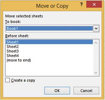
Figure2-17.Movecurrentsheettotheendorbeforeanothersheet
The MoveorCopydialog box has a check box option for creating a copy of the worksheet.
Selecting this option will make a duplicate worksheet of the one you right-clicked and it will place the new
copy in the location you specify in the Beforesheet: area of the dialog box. Excel names the
new copy the name of the original sheet plus it adds a number of the copy in parentheses. Figure 2-18 shows
that a copy of Sheet1 was moved to the end and named Sheet1 (2). If another copy was made of Sheet1 it would
be named Sheet1 (3). You can also rename the copied worksheets to something more meaningful.

Figure 2-18.Excel
adds a number to the end of the name of the copied worksheet
43
CHAPTER 2 ■ NAVIGATING AND WORKING WITH WORKSHEETS
■
NoteYou can also move
or copy worksheets to a different workbook.
Using Tab Buttons to Move Through
the Worksheets
If there are dots to the
left of the worksheet tabs this means that there are more worksheets to the
left of those
currently
showing. These dots are called ellipsis. If there is an ellipsis to the right
of the worksheet tabs this means that there are more worksheets to the right of
those currently showing. See Figure 2-19.
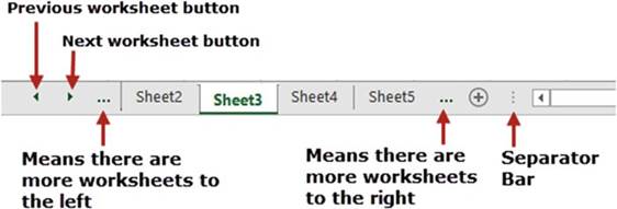
Figure2-19.Handlingworksheetsthataren�tvisible
Clicking the
Next worksheet button displays the tab for the next worksheet giving the result
as shown in Figure 2-20.

Figure 2-20.Sheet6
appears after clicking
the Next worksheet button
Clicking the Previous worksheet button twice at this point takes me back
two worksheet tabs. Since this is the first worksheet, the Previous worksheet
button is grayed out and the ellipsis is no longer displayed. See Figure 2-21.

Figure
2-21.Previous worksheet button
is grayed out and the left ellipsis
button is removed
If you want more room for displaying the worksheet tabs you can drag the separator bar to the right.
If you move your cursor over either the Previous or Next worksheet button a tooltip displays available
options. See Figure 2-22.
44
CHAPTER 2 ■ NAVIGATING AND WORKING WITH WORKSHEETS
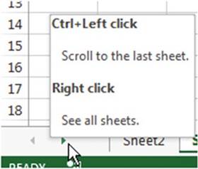
Figure 2-22.Tooltip displays when placing
cursor over the Previous or Next worksheet button
Holding down the Ctrl key while clicking the Previous worksheet button scrolls to the first worksheet.
Holding down the Ctrl key while clicking the Next worksheet
button scrolls to the last worksheet.
If you
right-click either the Previous or Next worksheet button, a dialog box displays
all of the worksheets from which you can activate the worksheet
you want. See Figure 2-23.
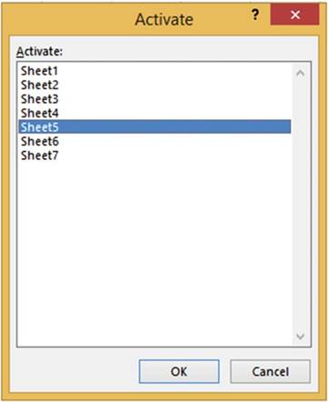
Figure2-23.AlloftheworksheetsappearintheActivatedialogbox
45
CHAPTER 2 ■ NAVIGATING AND WORKING WITH WORKSHEETS
This exercise covers how to move through the worksheet tabs and how to
hide and unhide worksheets.
1.
Create a new Workbook named WorksheetTabs.
2.
Right-click the Sheet1 tab. Select
Rename from the menu. Type Qtr1 Sales over
the text Sheet1.
3.
Click the New sheet button
three times.
4.
Double-click the Sheet2
tab. Type Qtr1 Expenses
over the text Sheet2. Press Enter
5.
Double-click Sheet3. Type Qtr1 Accts Receiv
over the text Sheet3. Press Enter
6.
Double-click Sheet4. Type Qtr1 Payroll over the text Sheet4.
7.
Insert four new worksheets. The first worksheets may no longer
be visible. Don�t
worry, they are still there.
Drag the separator bar
 �far to the right
so that you can see all of the worksheet tabs plus extra
space so that you can write longer
names on the tabs.
�far to the right
so that you can see all of the worksheet tabs plus extra
space so that you can write longer
names on the tabs.
8.
Name the new worksheets the same as the existing
ones except change
Qtr1 to Qtr2. Your tabs should look like those
in Figure 2-24.

Figure2-24.Yourworksheettabsshouldlooklikethese
9.
Drag the separator bar
�to the left so that you only see the first
five worksheet tabs.
10.
Click the Next worksheet button
 �twice so that you can view the next two tabs
that are hidden to the right.
�twice so that you can view the next two tabs
that are hidden to the right.
11.
Click the Previous worksheet button
 �so that you can view the tab that is hidden
to the left.
�so that you can view the tab that is hidden
to the left.
12.
Click Ctrl + the Next worksheet button
 �to view the last tab.
13.
Click Ctrl + the Previous worksheet button
 �so you can see the
first tab.
�so you can see the
first tab.
14.
Drag the separator bar
�to the right until
you can see all eight worksheet tabs.
15.
To activate a worksheet, right-click either the next Tab button
or the previous Tab button. Select Qtr1 Payroll from the Activate
dialog box. See Figure 2-25. Click
the OK button.
46
CHAPTER 2 ■ NAVIGATING AND WORKING WITH WORKSHEETS
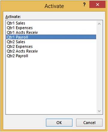
Figure2-25.SelectQtr1PayrollfromtheActivatedialogbox
16.
Next you will hide the worksheets for
both the Qtr1 and Qtr2 Accounts Receivable. Click the Qtr1 Accts Receiv tab, hold down
the Ctrl key, and click the Qtr2 Accts Receiv tab. Right-click the Qtr 2 Accts Receiv tab then
select
Hide.
17.
You will now bring back the two hidden worksheets. Right-click any one of the tabs and then select
Unhide� from the menu. Select
Qtr1 Accts Receiv
and then click OK. The worksheet is displayed back in its original position. Right-click any one of the tabs
and then select
Unhide� from the menu. Select
Qtr2 Accts Receiv and
then click OK.
18.
Let�s
remove the Qtr1and Qtr2AccountsReceivableworksheets
permanently from the workbook.
Click
the Qtr1 Accts Receiv tab, hold down the Ctrl key,
and click Qtr2 Accts Receiv tab. Right-click the Qtr2 Accts Receiv tab and select Delete.
19.
Move the Qtr1 Sales
tab after Qtr1 Expenses by clicking the Qtr1 Sales tab, dragging
it to the right until the down-facing arrow appears at the end of the Qtr1 Expenses tab,
and then releasing
your left mouse button. See Figure 2-26.
Move the Qtr2 Sales after the Qtr2 Expenses tab.

Figure2-26.DragQtr1SalesafterQtr1Expenses
47
CHAPTER 2 ■ NAVIGATING AND WORKING WITH WORKSHEETS
20.
Next,
you will copy a worksheet, but before you copy the worksheet you need to enter some data into the worksheet
being copied to verify that the copy worked. Click the Qtr1Expensestab. Enter some data in
several cells. Right-click the Qtr1 Expenses tab. Select Move or Copy. This brings up the Move or
Copy dialog
box.
In the Before sheet: area select Qtr1 Sales. Check the Create a copy at the
bottom
of the dialog box. See Figure 2-27. Click OK.
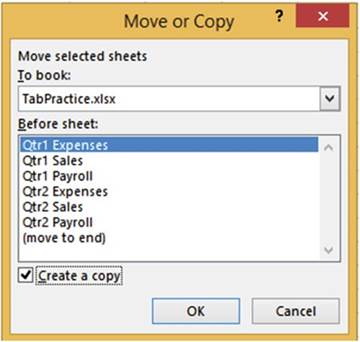
Figure 2-27. Select Create a copy
Worksheets Qtr1
Expenses and Qtr1 Expenses (2) should
contain the same data.
21.
Save the workbook as Chapter2Tabs.
As you learn more about worksheet functions and options, think about how
you will use the data. As you go through this book, you�ll learn more about planning and designing
workbooks and worksheets to meet your present and future needs.
Summary
You�ve learned a quick way
to move around worksheets and how to use special keyboard shortcuts to jump to different cells.
You�ve also worked with creating and customizing multiple worksheets within one workbook. In Chapter 3
you�ll create different types of data
and learn how to insert special characters and
adjust the size of columns and rows.
Included are shortcuts for entering the data to help you continue to use Excel in the
way that best suits your needs.
48
CHAPTER 3
Best Ways to Enter and Edit Data
In this chapter, you�ll
learn how Excel worksheets use three types of data: text, numeric, and date and
time. It is important to understand the different types of data. You�ll also
begin using special characters that you can�t find on the keyboard.
Excel has
several tools and features to make your data entry quick, efficient, and in the
format you want. Excel automatically determines how data is aligned
based on the type of data you enter. The data you enter can be
formatted by using various text, numeric, and data formats. If the data you
enter doesn�t fit in the cell the way you want, you can adjust the column widths
and row heights.
Excel�s
AutoCorrect feature can be useful for correcting commonly misspelled words,
misuse of capitalization, entering
special symbols that can�t be directly entered from the keyboard, and creating shortcuts for entering often
used
words or phrases.
The AutoComplete and Pick from Drop-down List features allow you to easily duplicate existing
column values. AutoFill can be used to create duplicate cells, enter a series of values, create a custom
list, or use a pattern that you taught it.
After
reading and working
through this chapter
you should be able to
�
Create the three types of data
�
Insert special characters
�
Change column widths and row heights
�
Correct typing mistakes
�
Use AutoCorrect to make corrections and to create
shortcuts for entering
words or phrases
�
Use AutoComplete to enter data
�
Use Pick from Drop-down List to enter data
�
Use AutoFill to create duplicate cells and create
a series
�
Create a custom
list
Data Types
There
are three types
of data that can be entered into a cell: text, numeric,
and date and time.
�
Text data. Text
data is also known as string data. The data can consist of a combination of letters, numbers, and some
symbols. Text data is
left-justified in a cell. You can�t use
text data in a formula.
�
Numeric data. A numeric
cell can only contain the characters shown in Figure
3-1.
� David Slager 2016�������������������������������������������� 49
D. Slager, Essential
Excel 2016, DOI 10.1007/978-1-4842-2161-7_3

CHAPTER 3 ■ BEST WAYS TO ENTER AND EDIT DATA
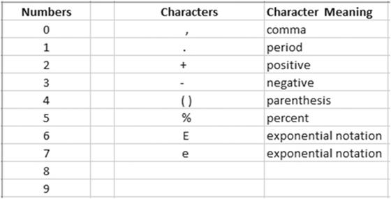
Figure 3-1.Only
these numbers and characters can be used in a numeric value
If any other
character or even a space is included in the cell, Excel treats the data as text.
Only cells that contain numeric values can be used in a formula. Numeric
data is right-justified in the cell.
�
Date and time data. Date and time data can be used for handling
dates, time, or a combination of the two. You can enter a date as January 16, 2005 or 01/16/05 or
01-16-2005, but how the date appears
in the cell depends on how the cell is formatted. Date and time data, like numeric data, is right-justified
in a cell.
■
Note� If you enter a date as January 15 2010 Excel will display it as text rather
than a
date because there is nothing to identify it as a date. If you place a comma after the day, Excel will be
able to identify it as a date and right justify
it.
The first
column in Figure 3-2
shows exactly
what text was entered into the cell; the second column shows how that entry would be
displayed in Excel. You could change how the date is displayed by changing its formatting which we will look
at
in a later chapter.
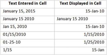
Figure3-2.Dateenteredinacellandhowit�sdisplayed
50
CHAPTER 3 ■ BEST WAYS TO ENTER
AND EDIT DATA
■
Note� When you are entering time into a cell, be sure
to place a space between
the time and entering AM or PM. The
time should be entered as 11:35 AM rather than 11:35AM. If you make the entry
without the space,
the time will be treated
as text data and it will be left-justified in the cell.
See Figure 3-3. You will not be able to perform
date and time functions on dates and times that are treated
as text.
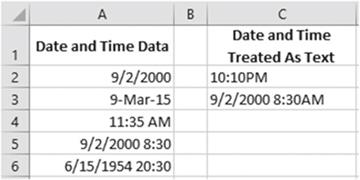
Figure 3-3.Entering time without a space makes it a text entry rather than a
date

In this exercise, create a new workbook and enter different kinds of data.
1.
Start Excel program. Create a
new workbook named Chapter 3.
2.
Type 5 Text in
cell A1. Press the Tab key. Because it is text, it stays
left-aligned.
3.
Type 12.75 in
cell B1. Press the Tab key.
Because it is numeric it moves to the right of the cell.
4.
Type 2/13 in cell C1. Press the Tab key. Because it
is a date it is right-aligned.
5.
Type 12:15 PM in cell D1. Press the
Tab key. Because it is a time
it is right-aligned.
6.
Type 5:10AM in cell E1. Press the Tab key. Because
you entered time without a space before AM, Excel left-aligned the time because
Excel thinks it is text.
7.
Type March 3 2014 in
cell F1. Press the Tab key. Because you entered a date without a comma after
the day, Excel left-aligned the date because Excel thinks it is text.
8.
Change the name on the Sheet1 tab to Data
Types
9.
Save the Workbook.
Inserting Special
Characters
If you want to enter a character that isn�t available on your keyboard, you can use one of Excel�s symbols
such as the greaterthanor equaltosign(≥) or the
lessthanor equaltosign(≤). The special characters can be accessed
by clicking the Ribbon�s Insert tab and then in the Symbols group click the Symbol button. See Figure 3-4.
51
CHAPTER 3 ■ BEST WAYS TO ENTER AND EDIT DATA
Figure3-4.SymbolbuttonislocatedintheRibbon�sSymbolsgroup
The Symbol
dialog box has two tabs, one for symbols and the other for special characters.
The Special Characters tab displays
commonly used symbols such as the copyright, trademark, different styles of
closing quotes, and so on. The
Symbols tab contains many more special characters, and that will be our focus
in this section.
The symbols
that are available on the Symbols tab depend on the selected font. Different
fonts have different symbols that they
can create. Some fonts have a lot more available symbols than others. For example, the generic (normal text)
option, shown in Figure 3-5,
provides a very large selection of characters.
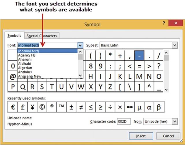
Figure
3-5.Use this when you need to enter
a character not available on your keyboard
The Recently
used symbols list displays the last 36 symbols that you have used. You can
insert one of the symbols or special characters into a cell by
clicking it and then clicking the Insert button.
52
CHAPTER 3 ■ BEST WAYS TO ENTER
AND EDIT DATA
Clicking the Insert button places the selected symbol in the current cell
but it doesn�t close the Symbol dialog box. This allows you to enter multiple symbols in the same cell
without having to reopen the Symbol dialog box. You may have to move the Symbol dialog box if it is
obstructing the view of the cell in which you are entering a symbol or special
character.
Clicking the down arrow to the right of the from: drop-down box reveals three categories of symbols to
select
from. See Figure 3-6.
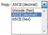
Figure3-6.Categoriesofsymbols
■
NoteThe three options
in Figure 3-6 are different ways your computer can represent data.
Unicode stands for Universal Code. Unicode code can display
over 16,000 symbols.
It is used to represent all the symbols
from all the languages around
the world.
ASCII stands for American Standard Code of Information Interchange. The ASCII format of creating symbols has
been around for a long time. It is capable of creating up to 256 different symbols. It uses symbols from the
United States and Western Europe.
ASCII(hex) codes are hexadecimal. They can use numbers
from 0 to 15
The Character
code is the numeric representation for the symbol you select. The Character code will be different
for the same symbol depending upon whether it is in a decimal or hexadecimal format. If you know the
character code for the symbol you wish to use, you can enter it to select the symbol.

In this exercise,
you add special characters to a spreadsheet. If you have closed the Chapter 3 workbook from the last
practice,
reopen it.
1.
Create a new worksheet. Rename the worksheet tab �Special Characters.�
2.
Click cell B2. On
the Ribbon, click the Insert tab. In the Symbols group, click the Symbol button.
3.
Select normal text from
the Font drop-down box, and then select ASCII (Decimal) from the from drop-down list in the
bottom right corner of the dialog box. Increase
the size of the Symbol dialog box until you can see all the symbols without
having to scroll.
4.
Click the � symbol. Notice the Character
code for the � symbol is 189. Click the Insert button. Move the Symbol dialog box so that you can see
cell B2.
53
CHAPTER 3 ■ BEST WAYS TO ENTER AND EDIT DATA
■
Note� Unfortunately you can�t
select another cell in your spreadsheet and then insert
another symbol. You must first close the Symbol dialog
box, select another
cell, and then reopen the Symbol dialog
box.
5.
Click the Close button on the Symbol dialog box.
6.
Type 25 in cell C2. Don�t press Enter. We will add a � after the 25.
7.
In the Symbols group on the Ribbon, click the Symbol button. Drag across (normal
text) in the Font drop-down box if it isn�t already highlighted. Type Ti then press the Tab key. This
will display the
symbols for the
Times
New Roman font.
Click
the � symbol then click the Insert button. Move the Symbol dialog box so that you
can see cell C2.
8.
Click the down arrow of the from drop-down box and select Unicode (Hex).
You�ll see a lot more symbols. Click the different symbols; as you do, notice that some of the symbols have
a letter
such A, B, C, D, E, or F in their character
code.
■
NoteWhen you selected Unicode
(Hex) a Subset drop-down box appeared in the upper right-hand corner.
Click some of the different
subsets.
9.
Close the Symbol dialog box.
10.
Click cell D2. In the Symbols
group on the Ribbon click the Symbol button.
Click the
� symbol in the Recently used symbols. Click the Insert button.
11.
Click the Special Characters tab in the Symbol dialog box. Double-click the Copyright
symbol.
Double-clicking a symbol does the same thing as clicking
it and then clicking the Insert button.
Move the Symbol dialog box so that you can see cell D2. Cell D2 should contain ��.
12.
Click the Symbols
tab. Click the down arrow for the Font drop-down box. Select Webdings. This font contains
some images that you might find useful.
Also look at the
Wingdings, Wingdings2, and Wingdings3 fonts.
13.
Close the Symbol dialog box.
14.
Click cell E2. You can enter most of the ASCII symbols directly
into a cell if you remember the character code. To enter a symbol directly into a cell
you would hold down the Alt key while you entered the character code on the numeric
keypad. The character code can
only be entered on the numeric keypad. Make sure the Num Lock key is on before you start entering
the number.
15.
Remember that the Character code for the � symbol is 189. Hold down the Alt key, type
0189, and then release
the Alt key. You should
see the � symbol. The extra 0 was needed
to make it a four-character number.
16.
Click the Save button
 �on the Quick
Access Toolbar (QAT).
�on the Quick
Access Toolbar (QAT).
54
How to Change
Column Widths
CHAPTER 3 ■ BEST WAYS TO ENTER AND EDIT DATA
When the text you type is
longer than the width of the column, the overflow characters are displayed in
the adjacent cell(s) to the
right if they do not contain any data. The characters may appear to be a part
of the adjacent cells but they are
not stored there. They are stored in the cell in which you entered them. In the following example, the name
Anthony
Bradtmueller displays across cells A3, B3, and C3 but the entire name is actually only stored in cell A3.
See Figure 3-7.

Figure 3-7. Text overflow
in next cell
If there are overflow characters and the adjacent cell to the right is not empty, then by default the
overflow characters are hidden as illustrated in Figure 3-8.
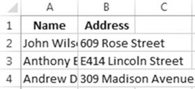
Figure3-8.Textishiddenbytextinnextcell
If you are entering
numeric data, the column will automatically expand
to fit the size of the number.
If the number that you are entering is the longest
value in the column and it contains
a decimal, then the decimal value may not be shown
in the cell. If you change the width of a column
that contains numeric
data, cells in that column will no longer
automatically adjust to the size of any new entries.
If a cell in a column that has had its size changed
contains numeric data that is longer than the width
of the cell, the cell will display # signs instead
of the numeric values. See Figure 3-9.
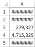
Figure 3-9.# signs mean the column isn�t wide enough to display
all the data
55
CHAPTER 3 ■ BEST WAYS TO ENTER AND EDIT DATA
The sight of
all these # signs always puts new users into a panic. They think that something
is horribly wrong with their spreadsheet.
If you click a
cell that contains # signs, the actual value will be displayed in the formula
bar. Just remember when you see # signs in a column the simple cure is to expand the
width of the column.
If you enter a very large
number into a cell you may see something like
 . This is exponential
notation. If you would rather view the value as a long number you can select the cell, click the
Number Format�s drop-down arrow located on the Home tab and then select which format you want the
exponential format converted to. See Figure 3-10. The number will probably be too big to display in the
cell; therefore you will need to widen the column width to view the number.
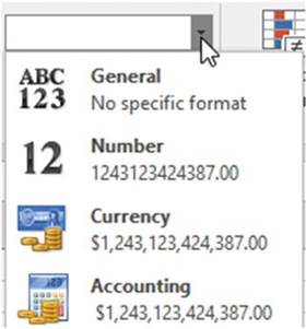
Figure 3-10.You can convert exponential notation
values to one of these formats
You can view
the column width by holding down your left mouse button while your cursor is on
the line between the column headings
(the cursor will turn into a double arrow). The default column width is 8.43 this allows for about 8 or 9
characters provided you are using the default font type of Calibri and font
size of
11.
See Figure 3-11.
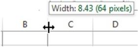
Figure 3-11. Check column width
Column widths can be changed by using the mouse to drag the column to the desired size. Expanding a column
width can be accomplished by holding down your left mouse button while your cursor is on the
line between the column heads, when the column width is displayed drag the line to the right to the desired
width. As you drag, Excel
shows you the width as well as a dotted vertical line that provides a visual
clue as to where the column border
will be changed to. See Figure 3-12.
56
CHAPTER 3 ■ BEST WAYS TO ENTER
AND EDIT DATA
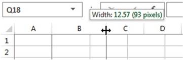
Figure 3-12. Adjust column width
The column
width can be shrunk as well as expanded. Drag the double
arrow to the left to shrink the size of the column.
You
can also change a column�s
width by performing the following steps:
1.
Right-click a column head and then select Column Width. The Column Width
dialog box opens (see Figure 3-13).
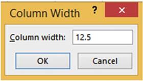
Figure 3-13. Changing column width
2.
Enter the desired width. You can enter any value between 0 and 255. Entering a width of 0 makes
the selected column(s) hidden.
3.
Click OK.
The Column Width dialog box can also be accessed by clicking the Home tab and then in the Cells
group click the Format button and then select Column Width. See Figure 3-14.
57
CHAPTER 3 ■ BEST WAYS TO ENTER AND EDIT DATA
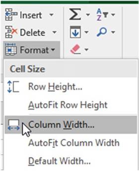
Figure3-14.Selectcolumnwidthfromformatbutton
Automatically Resize Column Widths
to Fit Number
of Characters in the Cell
You can have Excel
automatically adjust the size of the columns
to fit the number of characters in the cell. This can be accomplished by selecting the column heads for
those
columns whose width
you wish to change
and then double-clicking between any of the column
heads of the selected columns.
You can also perform an
AutoFit by right-clicking any of the selected columns and then selecting
AutoFitColumnWidthfrom the menu.
Changing the Column Width
for Multiple Columns
You can change the column width for more than one column at a time. The only difference between the methods
used for adjusting the width of multiple columns vs. a single column is that you need to select the column
heads for all the columns whose width you want to change. The column heads you select do not need to be
adjacent to each other. The following steps are an example of how to change the width of multiple columns at
the same time.
1.
Drag across
the column heads
of the columns whose width
you wish to change.
Figure 3-15 shows that column heads D, E, and F have been selected. Selecting a
column head selects the entire column.
58
CHAPTER 3 ■ BEST WAYS TO ENTER
AND EDIT DATA
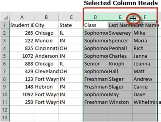
Figure3-15.Theentirecolumnsareselected
2.
Place your cursor between any of the selected column headings. The cursor
will turn into a double arrow as shown in Figure 3-15. Hold down the left mouse button and drag
it to the right to expand all of the selected columns or drag it to the left to
shrink all of the selected columns.
Now,
let�s apply some of the things learned
in this section.
In this exercise,
you create a new worksheet, create columns of data, and then modify the widths of those columns. If you have
closed the Chapter 3 workbook from the last practice,
reopen it.
1.
Create a new worksheet. Rename the worksheet tab �Column Widths.�
2.
Enter the Table 3-1 data into the worksheet starting in cell
A1. Do not adjust the column widths.
59
CHAPTER 3 ■ BEST WAYS TO ENTER AND EDIT DATA
Table3-1.Enterdataintoworksheet
|
Name
|
Address
|
Profession
|
|
Pyle, Gomer
|
308 Marine Barracks
|
Marine Private
|
|
Griffith, Andy
|
408 Mayberry Ave.
|
Town Sheriff
|
|
Presley, Elvis
|
215 Graceland
|
Rock Singer
|
|
Douglas, Lisa
|
509 Green Acres
|
Unusual Housewife
|
|
Adams, Mortisha
|
313 Spooky Lane
|
Strange Housewife
|
After entering the data your worksheet should look like Figure 3-16.
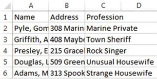
Figure3-16.Enterdatawithoutadjustingcolumnwidths
3.
Place your cursor between column heads A and B.
Drag your cursor to the right until the width is 16.43. See Figure 3-17.
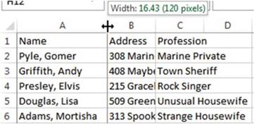
Figure3-17.Dragbetweencolumnheadstochangeacolumn�swidth
4.
Place your cursor between column heads A and B. Drag your cursor back to the left until the width
is 7. The text in column A is now partially hidden by the text in column B.
5.
Right-click column head
A and then select Column Width. Enter 8.43 for the column width. Click OK.
6.
Drag across column heads A, B, and
C to select all three columns.
7.
Double-click between column
heads B and C. Columns
A, B, and C adjust
to just fit the
longest text in their columns
as shown in Figure 3-18.
60
CHAPTER 3 ■ BEST WAYS TO ENTER
AND EDIT DATA
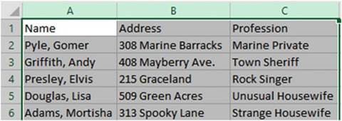
Figure3-18.Columnsadjustedtofitlongestcolumntext
8.
With column heads A, B, and C still selected, click the Ribbon�s
Home tab. In the Cells group click the Format
button. Select Column Width.
9.
In the Column
Width dialog box, enter 20 and click the OK button. The three columns
should each have a column width of 20.
10.
Click the Format
button again. Select AutoFit
Column Width. Columns
A, B, and C adjust
to just fit the longest
text in their
columns.
11.
Click the Save button
 �on the Quick Access Toolbar.
Now that you have learned to adjust the column width,
you�ll learn how to change
the height of the row so that you can view all of the text in a cell.
How to Change Row Heights
Changing the height of a row works the same as changing the width of a column. The row height is 15.00 by
default.
Changing row heights is accomplished by selecting the row or rows whose
height you want to change.
You select rows the same way you select
columns: click the number for a specific
row, drag on the numbers
to select adjacent
rows, or select
nonadjacent rows by holding down the Ctrl key while
clicking the row numbers (see
Figure 3-19).
After you have made your row selections, place the cursor
between the row head of one of the
selected rows and another row head then drag down to expand
the height of the row or up to shrink
it.
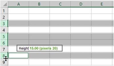
Figure
3-19.Select rows and then drag up or down to change the height of the selected
rows
61
CHAPTER 3 ■ BEST WAYS TO ENTER AND EDIT DATA
Double-clicking the line between
the numbers for the selected
rows adjusts the height of the row to accommodate the tallest text or object
in that row.
Another way to change
the row height
is to follow these steps:
1.
Select the row or rows that you want to change
2.
On the Home tab, in the Cells group,
click Format.
3.
From the menu you can select
Row Height or Autofit Row Height.
You can select
all of the rows in a spreadsheet by clicking the Select All button. You can
then adjust the height
of all rows by dragging up or down between any
row headers. The Select All button is located to the Left of the Column A header and above
the row 1 header. See Figure 3-20.
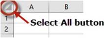
Figure 3-20. Select All button
This exercise uses the same spreadsheet you created for practicing changing
column widths. If you have closed the Chapter 3 workbook from the last practice,
reopen it.
1.
First we�ll create a copy of the Column Widths worksheet:
a.
Right-click the Column Widths worksheet
tab. Select Move or Copy.
b.
In the Move or Copy dialog box, click
(move to end) in the Before sheet list box.
c.
Click the Create a Copy check box and then click the OK button.
d.
Rename the Column Widths (2)
worksheet tab to Row Heights.
2.
Click Row Head 2. Hold down your CTRL key and click row
heads 5, 6, 9, and 12. Put your cursor between row heads 9 and 10 and drag down
until the size is about 22.5.
3.
Select cell A6. On the Ribbon, on the Home tab, in the Font group, type 22in the Font Size
text box then press Enter. The name Adams, Mortisha is now partially hidden. Double-click between column
heads A and B. This performs an AutoFit
adjusting the column width to accommodate the longest text in the column.
4.
Double-click between row heads 6 and 7. This performs an AutoFit adjusting the row height to
accommodate the tallest text
in the row.
5.
Click the Select All button. Put your cursor between any two row heads then drag down until the
height is 40.50. Double-click between any row head to make all rows AutoFit.
6.
With all rows still selected, right-click any cell and select Row Height from the menu.
Enter 25 for the Row Height
and then click OK.
7.
Click any cell to unselect
all of the rows.
8.
Click the Save button
 �on the Quick Access Toolbar.
62
CHAPTER 3 ■ BEST WAYS TO ENTER
AND EDIT DATA
You�ve learned how to adjust cell sizes by changing row heights and column widths. Next, you will learn
how to correct data entry errors.
Correcting Typing
Mistakes
Sometimes you make errors when entering data into a worksheet. If you do, it is easy to clear or correct what
you entered. There are several ways to clear or correct either some or all of the data from a cell. Let�s
look
at how to remove or change specific characters in a cell, how to clear data (and restore a cell to its
previous state) before accepting your data entry, and how to clear a cell for which you have accepted the
entry.
Changing Specific Characters
If you need to correct
specific characters in a cell, you have a couple of options depending on which characters they are and
whether you
have already accepted the data entry. First, you delete the character or characters you want to change and
then
type in the correct characters if necessary. Here are several ways to delete specific characters in a cell:
�
While still entering data in a cell, you can delete the last character or characters you entered
by pressing the Backspace key.
�
If you need to correct a character other than the last one(s) you typed, click just to the right
of that character and press Backspace.
�
If you have already
accepted the data in the cell, double-click in the cell to enter Edit mode and then click to the right of
the character you want to change or
use the left and right arrow keys to move the cursor to the
character you want to delete.
You
can correct typing
mistakes by doing
any of the following:
�
Remove the latest characters that you entered by pressing the Backspace key.
�
Clear an entry
before it has been accepted
by pressing the Esc(ape) key.
�
Clear an entry
before it has been accepted
by clicking the Cancel button
on the formula bar.
�
Clear the contents of a cell that has already been accepted by right-clicking a cell and selecting
Clear Contents.
If you only need to remove the latest characters that you entered, you can use the Backspace key.
Returning a Cell to Its Original Value
You can restore a cell to its original value if you have not yet accepted the data entry or if you have
accepted it but have not yet done anything else.
While you are
still entering data in a cell, you can clear what you�ve entered and restore
the cell to its previous
state. If it was an empty cell, you simply clear all the data. On the other
hand, if you changed the value in the cell, you clear the new entry and restore the cell�s original
value. Use either of the following techniques to restore a cell to its previous value before the new value
has been accepted:
�
Press the Esc(cape) key
�
Click the Cancel button
 �on the formula
bar
�on the formula
bar
63
CHAPTER 3 ■ BEST WAYS TO ENTER AND EDIT DATA
If you have already accepted the new data entry but have not yet done
anything else in the workbook, you can select the Undo button on the QAT (see Figure 3-21) or press Ctrl +
Z, which restores
the cell to its previous state: empty or containing the previous
value.
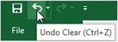
Figure 3-21. Undo button
Clearing the Contents of a Cell That Has Already Been Accepted
You can clear the contents
of a cell by right-clicking the cell and then selecting Clear Contents. You can
also select Clear Contents by
clicking the Ribbon�s Home tab and then selecting Clear > Clear Contents in
the Editing group.
In this exercise, you enter data in a new worksheet and then edit it. If you have closed the Chapter 3
workbook
from the last practice, reopen it.
1.
Add another worksheet and name it Edit
Data.
2.
Enter the data in Figure 3-22. For the date values in column C, let�s use three different formats:
a.
Enter the data in cell C2 as 10/15/1999.
b.
Enter the data in cell C3 as 6-15-2001.
c.
Enter the data in cell C4 as Jan 31, 2005.
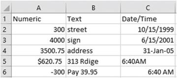
Figure 3-22. Enter this data
3.
Drag across column heads A, B, and C. Right-click one of the
selected column heads. Select Column Width. Enter 14. Click the OK button.
4.
Double-click cell A2 to enter
Edit mode. Change 300 to 550. Press Enter.
64
CHAPTER 3 ■ BEST WAYS TO ENTER
AND EDIT DATA
5.
Click cell B5. Press F2 to enter Edit mode. Change the word Rdige to Ridge.
Press Enter.
6.
Double-click cell C2. Change the date in the formula
bar to 10/15/2002. Click the Enter button (check mark)
 �in the formula
bar to accept the change rather than pressing Enter.
�in the formula
bar to accept the change rather than pressing Enter.
7.
Double-click
cell C3. Change the year to 1998 but don�t press
Enter. You decide
you really didn�t
want to make that change.
Press the Escape
key to return the cell to its original value.
Repeat this step again but instead of pressing the Esc key click the Cancel button
 �on the formula
bar.
�on the formula
bar.
8.
Right-click cell A6. Select Clear
Contents from the menu.
9.
Click cell B6. Click the Home
tab. In the editing group select
Clear > Clear Contents.
10.
Click the Save button
 �on the Quick Access Toolbar.
You have
learned how to handle any keying errors that you have made. Now, you�ll look at
Excel features that not only prevent you from making data entry
errors but at the same time increase the speed of entering the data.
Shortcuts for Entering
and Correcting Data
Excel provides the AutoComplete, Pick data from drop-down list, AutoFill, and AutoCorrect methods to speed up
data entry and ensure that your data has been entered without errors.
Using the AutoCorrect Feature
Excel�s AutoCorrect feature
can speed data entry as well as help prevent errors from being entered into
your worksheet by automatically
adjusting entries or by fixing common typing errors as they are being entered. Excel�s AutoCorrect feature
is useful
for the four following situations:
�
Correcting commonly
misspelled words. If you spell the word �achieved� as �acheived� Excel
will automatically correct
it.
�
Enteringspecialsymbolsthatcan�tbedirectlyenteredfromyourkeyboard.If
you type
(tm) Excel
will automatically convert
it to the trade symbol �.
�
Creating
shortcuts for entering words or phrases that you enter often. You could enter your initials and
Excel would
convert it to your full name.
�
Misuse
of capitalization. If you type monday, Excel corrects
it to Monday.
■
Note� Microsoft office applications share the same AutoCorrect Options
as Excel; therefore any changes, additions, or deletions you make to the AutoCorrect options in Excel
will affect those
in other Microsoft office applications and vice versa.
65
CHAPTER 3 ■ BEST WAYS TO ENTER AND EDIT DATA
In this exercise, you experience Excel�s
default AutoCorrect functionality and then look at how you can modify it for your own preferences. If you
have closed the Chapter 3 workbook from the last practice,
reopen it.
1.
Add another worksheet and name it AutoCorrect.
2.
In cell A1 type abbout then press the Tab key.
Excel corrects it to about
3.
In cell B1 type (c) then
press the Tab key.
Excel converts (c) to a copyright symbol
4.
In cell C1 type (r) then
press the Tab key. Excel
converts (r) to a registered symbol.
5.
In cell D1 type your name starting with two capital letters
such as DAvid and then press the Tab key.
Your results should look similar to those in Figure 3-23.
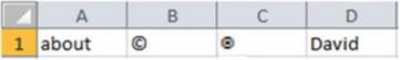
Figure3-23.ResultsofusingAutoCorrect
Add Items
to the AutoCorrect List
Now that
you�ve seen how AutoCorrect works by
default, you can add new items to AutoCorrect:
1.
On the Ribbon click the File tab.
2.
Click Options in the left pane.
This opens Excel
Options. See Figure
3-24.
66
CHAPTER 3 ■ BEST WAYS TO ENTER
AND EDIT DATA
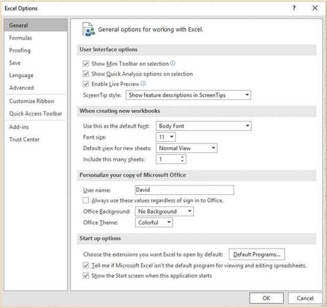
Figure 3-24. Excel Options
3.
Click Proofing in the left pane.
4.
In the right pane under AutoCorrect Options
click the AutoCorrect Options button.
This brings up the AutoCorrect
dialog box. See
Figure 3-25.
67
CHAPTER 3 ■ BEST WAYS TO ENTER AND EDIT DATA
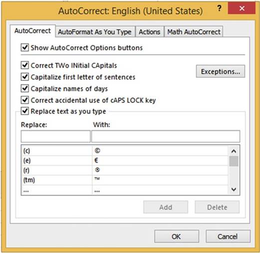
Figure
3-25.AutoCorrectdialogboxwithAutoCorrecttabselected
You can see that there is an option for Correct Two Initial
Capitals. This is what corrected
your name entry.
There are also options for capitalizing the first letter
of sentences, names of days,
and correcting the accidental use of the Caps Lock key.
Look at the bottom half of the tab, there is a two-column table.
The left column has a heading of Replace: and the right column has a heading
of With: Entries in the Replace:
column are replaced
with those in the With:
column. You used three entries
in the table. You entered
(c) in a cell and it was replaced with the copyright symbol �. You entered
(r) and it was replaced
with the registered symbol �. If you scroll
down in the table you can see that abbout will
be replaced with about which you have already
done.
5.
Scroll through the table and see what other corrections are available.
6.
Enter tommorrow in the Replace text box. Enter tomorrow in the With text box. Click
the Add button. The new AutoCorrect item is added to the list. See Figure 3-26.
68
CHAPTER 3 ■ BEST WAYS TO ENTER
AND EDIT DATA
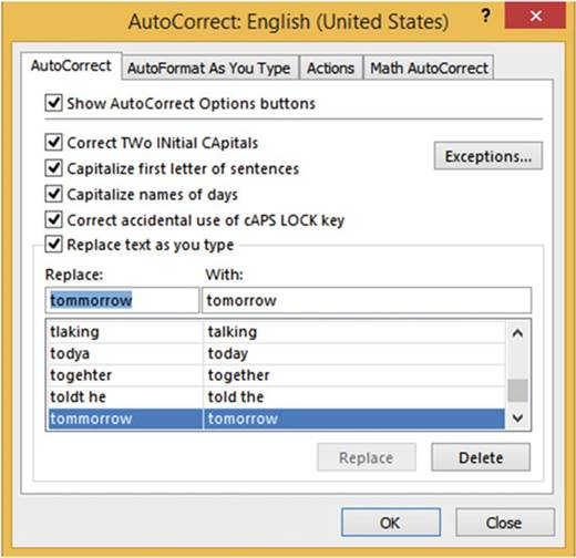
Figure3-26.ThenewAutoCorrectitemhasbeenadded
7.
Type your initials
in the Replace text box over the existing text. Enter your full name in the With text box over the existing
text. Click the Add button.
8.
Enter phoneA in the Replace text box. Enter (380)599-1275
in the With text box. Click the Add button.
You could make phone numbers for your home phone and your cell phone.
9.
Enter any other corrections or shortcuts you would like to make.
This could be a big time saver.
If you often enter your company name,
you should create
a shortcut for it or any other
text that you use often.
10.
Click the OK button in the AutoCorrect dialog box. Click the Cancel
button in the Excel Options
dialog box.
11.
Type tommorrow in cell A2 then press the Enter key�Replaced with
tomorrow
12.
Type your initials in cell A3
then press the Enter key�Replaced with your full name
13.
Type phoneA in cell A4 then press the Enter key�Replaced with
(380)599-1275
14.
Put your Caps Lock on. Hold down your shift key while typing an E. Let go of your shift key
and type xcel. Cell
A5 should now contain eXCEL.
Press the Enter key.
Cell A5 should now contain
Excel. This was corrected by
the Correct Accidental use of cAPS LOCKkey option.
69
CHAPTER 3 ■ BEST WAYS TO ENTER AND EDIT DATA
Delete
items from the AutoCorrect list
1.
On the Ribbon, click the File tab.
2.
Click Options in the left pane.
3.
Click Proofing in the left pane of Excel Options.
4.
In the right pane, click the AutoCorrect Options button.
5.
Type phoneA in the Replace text box; as you do so the list will jump to the letters
you are entering. When phoneA is highlighted in the list,
press the Delete
button.
6.
Remove the shortcut you created for your initials. Remove any other shortcuts you created that you
want deleted.
7.
Click the Close button on the AutoCorrect dialog box. Click
the Cancel button
on the Excel Options dialog
box.
8.
Click the Save button
 �on the Quick Access Toolbar.
You have just
used Excel�s AutoCorrect feature to correct misspelled words and to create
quick shortcuts for entering words or phrases. Next you will use the
AutoComplete feature to duplicate data that already exists in
the column.
Using AutoComplete to Enter Data
The AutoComplete feature is automatically set up; there
are no buttons to click
or commands to be entered. The
AutoComplete feature compares
the entry you are making
to entries that already exist
in the same column. As you are typing your entry, Excel
looks for a word that starts with the same letters as the word you are
entering. If it finds an existing word in the column that starts with the same letters you have entered
so far, it places that word in the active
cell. See Figure
3-27

Figure 3-27.AutoCorrect automatically added the letters rt after you typed the
letters sma
The first two letters are the same for all words in the column. When you type the letter a in the
second entry for the word smart, Excel sees that there is only one word that starts with sma
so it places the word smart in the cell. You can accept the word by pressing the Enter key, the
tab key, or the down arrow key or you can clear the cell by pressing Esc(ape).
Only after typing the second ain the word savant in Figure 3-28 is there a word that matches all the
letters typed so far. You can accept the word by pressing the Enter key, the tab key, or the down arrow key
or you can clear the cell by pressing the Esc key.
70
CHAPTER 3 ■ BEST WAYS TO ENTER
AND EDIT DATA
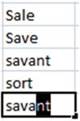
Figure 3-28.AutoCorrect automatically added the letters nt after you typed sava.
■
Note� AutoComplete does not work if there is an empty cell above the current
cell.
Pick from Drop-down List
The Pick from Drop-down List feature is similar to the AutoComplete feature. The Pick from Drop-down
List like the AutoComplete feature,
lets you use entries that already exist
in the column. The Pick from
Drop-down List lets you select from a list of existing
entries that are automatically sorted
for you. The list can be accessed
by right-clicking the cell and selecting Pick from Drop-down List or by pressing Alt + Down
Arrow. See Figure
3-29.
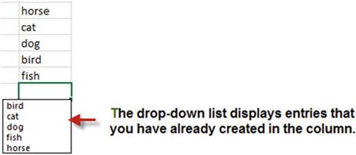
Figure 3-29. Pick from Drop-down
List
■
Note� Pick from Drop-down List does not work if there is an empty cell above the
current cell.
Let�s use Autocomplete and Pick
From Drop-down List to add text.
AutoComplete
Let�s see AutoComplete in action in this exercise. If you have closed the Chapter 3 workbook from the last
practice, reopen it.
71
CHAPTER 3 ■ BEST WAYS TO ENTER AND EDIT DATA
1.
Add another worksheet and name it AutoComplete.
2.
Type the names in column A as
shown in Figure 3-30.

Figure3-30.Enternamesinworksheet
3.
Type the letter
C in cell A6. The name Carl appears
in the cell because there
is no other name that starts with C.
4.
Type Da in cell A7. Since there are two names that start with a D in the column,
Excel can�t find a unique one at this point.
Type a v after the Da. Only one name starts with Dav so Excel
enters David in the cell.
Press Enter.
5.
Type Mar in cell A8. Since there are two names that start with Mar in the column, Excel
can�t find a unique one at this point.
Type a t after the Mar. Only one name starts with Mart so Excel enters Marten in the cell.
Pick from
Drop-down List
In this
exercise, you use the Pick from Drop-down List feature.
1.
Right-click in cell A9 and then
select Pick from Drop-down List from
the menu.
Notice that your entries are displayed in alphabetic
order and no duplicates are displayed. See Figure 3-31
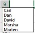
Figure 3-31.Entries are in alphabetic order and there are no duplicate names
2.
Click David. Press the Enter key.
3.
Press Alt + Down Arrow. Select Marten. Press the Enter key.
4.
Click the Save button
 �on the Quick Access Toolbar.
72
CHAPTER 3 ■ BEST WAYS TO ENTER
AND EDIT DATA
The AutoComplete feature and the Pick from Drop List both provide a quick way of creating duplicate data in a
column. The AutoComplete feature automatically provides suggestions for you to select from
as you type. The Pick from
Drop-down List displays all the entries you have made thus far in the current column and
then lets you pick one from the list to duplicate. Next, you will look at how
the AutoFill feature not only lets you duplicate data but also creates
repeated patterns of data.
AutoFill
The AutoFill feature allows
you to fill cells automatically with data that follows a pattern or that is based on data
in other cells. It can also be used to create duplicate cells, enter a series of values, and create a custom
list.
Use AutoFill to Create Duplicate Cells
You can copy
values in one cell to additional cells by dragging the AutoFill Handle in the
direction that you want.
The AutoFill Handle is a small black square at the bottom right corner of the
active cell (Figure 3-32). Placing the cursor over the AutoFill
Handle turns the cursor into a plus sign (Figure 3-33).
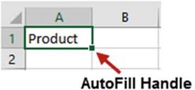
Figure 3-32. AutoFill Handle
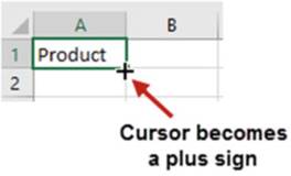
Figure 3-33.Cursor becomes a plus sign when moved
over AutoFill Handle
A ToolTip is displayed as you drag the AutoFill Handle across other cells indicating the value that will be
placed in that cell when you release the mouse button (Figure 3-34).
73
CHAPTER 3 ■ BEST WAYS TO ENTER AND EDIT DATA
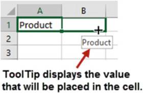
Figure 3-34. ToolTip
Figure 3-35 shows the result
of dragging the AutoFill Handle
from A1 through
D1.
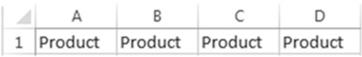
Figure3-35.ResultsofdraggingAutoFillHandle
You can drag the AutoFill Handle across as many cells as you like and you can drag it in any direction.
Figure 3-36 shows the result
of dragging the AutoFill Handle
up.
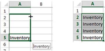
Figure3-36.ResultofdraggingAutofillHandleup
Using AutoFill to Enter a Series of Values
AutoFill, in addition to
being able to duplicate cell values, can also be used to create a series of
repeating data lists. Excel has
built-in data series related to days, months, years, numbers, and so on. For
example, you can enter Monday into a
cell then use the Autofill Handle to automatically enter the other days of the
week in adjacent cells. As you
are dragging the AutoFill Handle, Excel shows you what is going to be placed in
that cell when you have finished
dragging (see Figure 3-37).
74
CHAPTER 3 ■ BEST WAYS TO ENTER
AND EDIT DATA
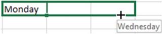
Figure 3-37.As you drag across cells using the AutoFill Handle Excel shows what it
will place in that cell
It doesn�t
matter what day of the week you start with. If you drag across more than seven
cells, the days will start repeating. You can also use a
three-character abbreviated day.
Dragging across the cells as shown in Figure 3-38 will result in the series shown in Figure 3-39.

Figure 3-38.Using
the AutoFill Handle on a day of the week, it will repeat that day every seven cells

Figure3-39.ResultofdraggingAutoFillHandlestartingwithFri
Excel knows
that there are four quarters in the year. If you type Quarter 1 then use the AutoFill
Handle to create a series, Excel
will go from Quarter 1 to Quarter 4, and then it will repeat the pattern
starting with Quarter 1. See Figure 3-40.

Figure3-40.SeriesstartingwithQuarter1
You
can also use the abbreviation Qtr for Quarter.
If you have a word before a number in a cell, Excel will increase the number by 1 for each cell in the
series. See Figure 3-41.

Figure3-41.SeriesstartingwithSection2
Teaching Excel to Create an AutoFill Pattern
You can teach Excel
a pattern. If you want to display
every third number,
you can enter
a value of 1 in a cell and
a 4 in the next cell. You would select
both cells and then, using
the AutoFill Handle,
drag across as many cells as you want to include
in the pattern. This would
produce a pattern
of 1, 4, 7, 10, and so on.
If you want to display a series of adjacent cells
with 15-minute intervals, select the first
two cells to teach it
the pattern (Figure
3-42) and then drag the AutoFill
Handle for as many cells
as you want to include
in the pattern. When you finish
dragging the result
will be as shown in Figure 3-43.
75
CHAPTER 3 ■ BEST WAYS TO ENTER AND EDIT DATA
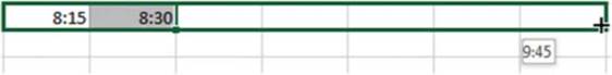
Figure 3-42.Select two adjacent cells to teach
Excel an AutoFill pattern

Figure 3-43.Result of dragging AutoFill Handle
using two adjacent times
Using the AutoFill
Options Button
When you have finished using the AutoFill Handle to copy a cell or create a series, an Autofill Options
button
appears to the bottom right of the last selected cell.
Clicking the Autofill Options button brings up three or more options if you used the AutoFill Handle to copy
a cell that contains alpha data.
Clicking the Autofill Options button brings up three options when copying alpha data in a horizontal
format. The default is Copy Cells. See Figure 3-44.
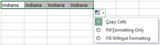
Figure3-44.OptionsavailablefromAutoFillOptionsbutton
Clicking the Autofill Options button brings up four options when copying alpha data in a vertical
format. The default is Copy Cells. See Figure 3-45.
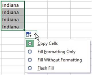
Figure3-45.AutoFilloptionswhencopyingdatavertically
76
CHAPTER 3 ■ BEST WAYS TO ENTER
AND EDIT DATA
Clicking the Autofill Options button brings up four or more options if you used the AutoFill Handle to copy
numeric data. See Figure 3-46.
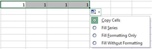
Figure3-46.AutoFilloptionswhencopyingnumericdata
Clicking the Autofill Options button brings up many options if you used the AutoFill Handle to copy
Date data. See Figure 3-47.
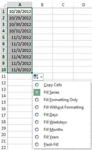
Figure3-47.AutoFilloptionswhencopyingdatedata
77
CHAPTER 3 ■ BEST WAYS TO ENTER AND EDIT DATA
Selecting the Copy Cells option would revert the series you
just created back to copies of the original cell you used for
making the series. The ten cells would all contain 10/28/2012
The Fill Formatting Only option will only copy any formatting that you have applied to the original
cell(s) to the cells you dragged across
with the AutoFill
Handle. It will not place
any data into the cells.
The Fill Without
Formatting option will copy the data or create a series from the original
cells but it will
not apply any formatting from the original
cells to the data you created using
the AutoFill Handle.
The next practice, Exercise
3-9, illustrates the Autofill Options.
Create an Autofill
Custom List
In addition to using
Excel�s built-in data series you can create your own. If you find yourself
constantly entering the same series of
values, then you should create your own data series to speed up your entries.
The data series can be created
in the Custom Lists dialog box which can be accessed by clicking the Ribbon�s
File tab, selecting Options in
the left pane, selecting Advanced in the left pane, scrolling the right pane
until you see the General section,
and then clicking the EditCustomListsbutton. See Figure 3-48.
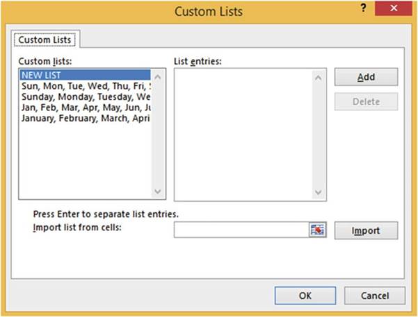
Figure3-48.CreateyourownCustomListintheCustomListsdialogbox
You type the
new data series in the List entries box. Then click Add to add the data series
to the Custom
lists box. You
can also create a new custom list by selecting the cells on your worksheet and
clicking Import in the Custom Lists dialog box.
78
CHAPTER 3 ■ BEST WAYS TO ENTER
AND EDIT DATA

In this exercise, you practice using
AutoFill techniques. If you have closed the Chapter 3 workbook from the last practice, reopen it.
1.
Add another worksheet and name it Custom
Lists.
2.
Type Tuesday in cell A1. Using the AutoFill
Handle drag to the right.
As you drag past each cell, notice
what Excel is going to place in that cell. Drag to cell J1.
3.
Type Qtr1 in cell A2. Using
the AutoFill Handle drag to the
right to cell F2.
4.
Type 10:00 in cell A3. Using
the AutoFill Handle drag to the right
to cell F3.
5.
A series can be created
vertically as well as horizontally. Type Sep in cell A4. Using
the AutoFill Handle drag down to cell A14.
6.
Type June in cell H5. Using the AutoFill
Handle drag to the left to cell C5. You should now have a series of January through
June.
7.
Type Store 3 in
cell C7. Using
the AutoFill Handle
drag to the right to cell G7. You should
now have a series of Store 3 through Store
7.
Teach
AutoFill a Pattern
You can
teach AutoFill to use a consistent
pattern.
1.
Type 1 in cell C9. Enter
a 3 in cell D9. Drag across
both cells. With both cells selected drag the AutoFill
Handle through cell H9.
2.
Enter a 1 in cell C10. Enter a 4 in cell D10. Drag across both cells. With both cells selected
drag the AutoFill
Handle through cell H10.
3.
Enter 8:30 in cell C11. Enter 9:00 in cell D11. Drag across both cells. With both cells
selected drag the AutoFill Handle
through cell H11.
Use the
Autofill Options Button
Try using
the AutoFill Options button:
1.
Type Section 1 in
cell A16 and Section
2 in Cell B16. Select
both cells. Press
Ctrl
+ B + I to bold and italicize both cells. With both cells selected drag the AutoFill Handle through cell F16.
2.
Click the Autofill Options button. See Figure 3-49.
79
CHAPTER 3 ■ BEST WAYS TO ENTER AND EDIT DATA
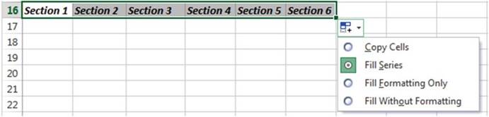
Figure 3-49. AutoFill options
3.
Select Copy Cells. Instead of filling a series, the original Section
1 and Section 2 are copied to the other
cells. See Figure
3-50.

Figure 3-50.The selected two cells are copied to the other cells
Holding down the Ctrl key as you drag the AutoFill Handle
is a way of forcing
Excel to copy values rather
than create a pattern without
having to use the Autofill
Options button.
4.
Press Ctrl + Z to undo the change.
5.
Select cells A16 and
B16. Hold down the Ctrl key while you drag the AutoFill
Handle through cell F16.
6.
Press Ctrl + Z to undo the change.
7.
Select cells A16 and B16. With both cells selected
drag the AutoFill
Handle through cell F16.
8.
Click the Autofill
Options button. Click Fill Without Formatting. The cells that were filled
with the AutoFill
Handle lose their formatting. See Figure 3-51.

Figure3-51.Thevaluesinthecellsarecopiedbutnotanyformatting
9.
Click the Autofill
Options button. Click Fill Formatting Only. The data in the cells that were filled
with the AutoFill
Handle are cleared
but the Bold and Italicize
formatting still apply
to those cells.
Type the word Sales in cell D16. The word Sales
is bolded and italicized.
10.
Type 2/1/2013 in
cell A18. Drag the AutoFill
Handle through cell F18. Click the
Autofill Options button.
11.
Select Fill Weekdays. The list skips over Saturday and Sundays.
80
CHAPTER 3 ■ BEST WAYS TO ENTER
AND EDIT DATA
12.
Click the Autofill
Options button. Select
Fill Months. The list creates a series of months with the same day. See Figure 3-52.

Figure 3-52.The Autofill option Fill Month automatically adjusts
the month and year but leaves the day the same
13.
Click the Autofill
Options button. Select Fill Years. The list creates
a series of years with the same month and day. See Figure 3-53.

Figure 3-53.The
Autofill option Fill Years adjust
the year but keeps the month and day the same
14.
Click the Autofill
Options button. Select Fill Without Formatting. Excel�s calendar starts
with the date January 1, 1900 and since the list is unformatted it displays the number of days since
January 1, 1900.
See Figure 3-54.

Figure 3-54.The Fill Without
Formatting option displays
the number of days for that date since January
1, 1900
15.
Click the Autofill
Options button. Select
Copy Cells. The list consists of the same copied cell.
See Figure 3-55.

Figure3-55.UsingtheoptionCopyCells
16.
Click the Save button
�on the Quick Access Toolbar.
You have
finished covering all of Excel�s shortcuts for entering data. In this section
you learned how to copy
data and repeat patterns. You even learned how to create your own patterns. In
the next section you�ll learn
how to make comments for the data in a cell. Comments serve as a memory aid for
you or others to remember
where the data came from or what it represents.
81
CHAPTER 3 ■ BEST WAYS TO ENTER AND EDIT DATA
Creating, Viewing, Editing, Deleting, and Formatting Cell Comments
You can attach a comment to
any worksheet cell. A comment could be information that you want to share with others or just to help
yourself
remember�such as how or why a formula was entered, where the data came from, what data still needs to be
entered, and so on. You can think of a comment as a sticky note. Every place in the worksheet that you would
want to place a sticky note to help you remember something, you can create a comment. Comments are
actually better than sticky notes because they won�t fall off the sheet and they are easily editable. Cells
that
contain comments are easily identified by a red triangle in the upper right corner. The comments can be
viewed by
moving your cursor over the red triangle. See Figure 3-56.
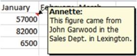
Figure3-56.Cellswithcommentshavearedtriangleinupperrightcorner
The buttons that handle comments are located in the Comments group of the Review tab. See Figure 3-57.
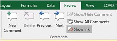
Figure3-57.TheRibbon�sCommentsgroup
If there are no comments
in the workbook, the Delete,
Previous, and Next buttons are grayed out.
The Show Ink button in the Comments group does
nothing if you have a desktop or laptop computer. It is only functional for
creating annotations on Tablet PCs where it allows users to create comments,
shapes, highlights, and text on the
screen with a stylus.
How to Add a Comment
Few people take the time to
enter comments into their Excel worksheets. Adding comments is time well spent. I think it is very important
to
get beginners off to a good start and so I am presenting comments here in the data entry chapter because it
should be a part of your normal entry routine.
1.
Click the cell to which you want to attach a comment.
2.
Click the Review
tab. In the Comments group,
click the New Comment button or right-click the cell and select Insert
Comment.
82
CHAPTER 3 ■ BEST WAYS TO ENTER
AND EDIT DATA
3.
Type the comment in the comment box.
4.
Click outside the comment box.
How to View a Comment
Follow these steps to view a comment:
1.
Move your cursor over a red triangle.
2.
If the workbook contains
more than one comment. You can click the Previous or
Nextbutton to move from comment to comment.
3.
By Default, comments remain hidden until you move your cursor over the red triangle. If you
want a comment to remain visible even when you move your cursor away from
the red triangle, then click the Show/Hide comment button. The button is
available from the Ribbon or by right-clicking the cell and selecting it from the
context menu.
How to View all the Comments at the Same Time
You
also can view all comments
by doing the following:
1.
Click the Review tab.
2.
In the Comments group, click Show All Comments.
How to Change the Default Name for Comments
By default Excel places your username
in the comment. The name can be removed and changed by doing
the following:
1.
To delete the username
in a comment, select the name and press the Delete key.
2.
To change the default name for all comments, click the File tab and then click Options in the left
pane.
3.
Select Generalin the left pane
4.
In the PersonalizeyourcopyofMicrosoftOfficegroup, type
the name you wish to use in the UserNametext box.
5.
Click the OK button.
■
Note� You might not use a worksheet for months and then things
you thought you would remember
you no longer do. If you are like me and write
notes to yourself
on a piece of paper,
you will probably
lose it and then spend hours looking
for it. So, make life easy on yourself and use comments
in Excel frequently.
83
CHAPTER 3 ■ BEST WAYS TO ENTER AND EDIT DATA
Editing and Deleting Comments
If you right-click a cell that contains a comment, the context menu no longer has an Insert
Commentoption but instead contains an Edit Commentand a Delete Commentoption. Clicking
the Edit Comment brings the comment up for editing. Make the changes you wish then click outside the comment
to update the comment with the changes. Clicking Delete Comment removes the comment without asking for any
verification.
Printing a Comment
Comments do not print by default. The option to print comments is located on the Page Setup dialog box. The
Page Setup dialog box can be accessed by clicking the Page Layout tab on the Ribbon, and then clicking the
dialog box launcher of the Page Setup group. It can also be accessed by clicking on the File tab, then
selecting Print, and then clicking the PageSetuplink. Once you are in the Page Setup dialog
box, select the Sheettab. From the comments drop-down box you can select either to have the comments
printed at the end of your worksheet data or to be printed as they appear in your worksheet. See Figure
3-58.
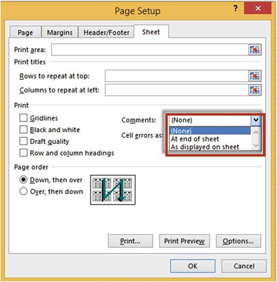
Figure3-58.Selectwhereyouwantcellcommentsprinted
84
CHAPTER 3 ■ BEST WAYS TO ENTER
AND EDIT DATA
In this exercise, you add, work, and print comments.
1.
Start a new worksheet named
�Comments.�
2.
Right-click any cell. Select InsertComment. Type anything you wish for a comment.
3.
Do the same for three more cells. You should now have four cells with red triangles in them.
View the
Comments
1.
Move your cursor over each comment to view it. Click one of the cells that contain a
comment.
2.
On the Ribbon,
on the Review tab, in the Comments
groups, click the Show/Hide
Comment button. The comment is displayed.
3.
Click the Show/Hide Comment button
again. The comment is now hidden.
4.
Click the Next button in the Comment group. Click the Next button twice more. Click the
Previous button twice.
5.
Click the Show All Comments button. All four comments are displayed. Click the
Show All Comments button again. The
four comments are now hidden.
Edit a
Comment
1.
Click the cell of your first comment. Click the Edit Comments button in the Comments group.
2.
Type some more text in the comment. Click
somewhere outside the comment.
Delete a
Comment
1.
Click one of the cells that contains
a comment.
2.
Click the Delete button. The comment is removed. The cell no longer contains a red
triangle.
Print the
Comments
Only the comments that are currently displayed on the worksheet will be
printed.
1.
Click the Show All Comments button
to display all of the comments at once.
2.
Click the File tab on the Ribbon. Select
Print from the left pane.
3.
Click Page Setup
located at the bottom of the Settings
options. This brings
up the Page Setup dialog
box.
4.
Click the Sheet tab on the Page Setup dialog box.
5.
Click the down arrow of the Comments drop-down box. This
displays three options. See Figure 3-59.
85
CHAPTER 3 ■ BEST WAYS TO ENTER AND EDIT DATA
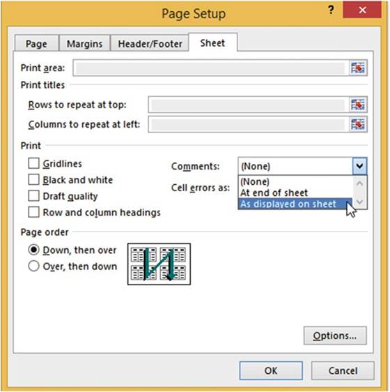
Figure3-59.Selectwherecommentsaretobeprinted
Selecting None will display no
comments in the printout.
Selecting At end of sheet will
print the comments
after the spreadsheets have printed. The printout shows the comments
along with the cell address
of each comment. See Figure
3-60.
86
CHAPTER 3 ■ BEST WAYS TO ENTER
AND EDIT DATA

Figure3-60.ResultofselectingAtEndofSheet
Selecting As displayed on sheet prints the comments within the data exactly as they appear on the
spreadsheet. See Figure 3-61.
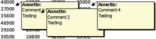
Figure 3-61.Result
of selecting As displayed on sheet
87
CHAPTER 3 ■ BEST WAYS TO ENTER AND EDIT DATA
Summary
This chapter covered the various data types and how those types can affect how your data looks and how it is
adjusted within a cell. It also covered different ways of entering and editing data.
This chapter focused on knowing how to change the size and appearance of columns and rows in the
worksheet and learning how to use special characters, as well as Excel�s AutoCorrect function. You
can
create, edit, delete, and print comments that you add to a cell.
Excel�s AutoCorrectfeature can be useful for such things as correcting
commonly misspelled words, misuse of capitalization, entering special symbols that can�t be directly
entered from the keyboard, and creating shortcuts for entering often used words or
phrases.
The
AutoComplete and Pick from Drop-down List features allow you to easily
duplicate existing column values.
In Chapter 4, you�ll learn how to use more complex data and cell formatting features. There are also a
variety of options for presenting and formatting numeric data including those for accounting purposes.
You�ll also begin using the mini toolbars and context menus, which provide more shortcut options particular
to what you are working on.
88
CHAPTER
4
Formatting and Aligning Data
You�ll now learn how to refine the way your worksheets look on screen and in print. Excel provides many great
options to establish a style for worksheets and the workbook
as a whole that is distinctive and consistent.
After reading and
working through this chapter you should be able to
�
Format data and cell backgrounds
�
Create cell borders
�
Check which formats have been applied to the
current cell
�
Align data
�
Copy the formatting from one cell to other
cells
�
Format numeric data
�
Use Context Toolbars menus
Reasons for formatting data include emphasizing certain entries (e.g., totals) and making the worksheet more
visually appealing
and easier to understand (e.g., by using colors to visually segment
rows and columns).
This helps keep information organized
for both the person creating
the worksheet and others who use it for analysis
and reports. Formatting can also be used to change how you display
numeric data (with dollar signs, commas, decimals,
percent, etc.). Formatting is also used to align data. You can use Excel�s Format Painter to copy all the
formatting applied to a cell to other cells. You can create cell borders to separate different
areas or to highlight a particular area on your worksheet.
Formatting Your
Text Using the Font Group
The Font group located on the Home tab has options for such things as changing
the font, size, color, and so
on. Figure 4-1 shows the formatting command buttons in the Font group. We will discuss
each of these in the following text.
89
CHAPTER 4 ■ FORMATTING AND ALIGNING
DATA
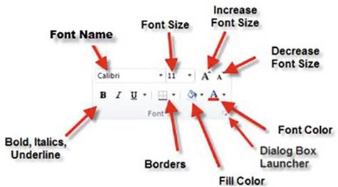
Figure4-1.Fontformattingcommandbuttons
Using Bold, Italics,
Underline, and Double Underline
You can use any combination of bolding, italicizing, or underlining on your text. Selecting one or any
combination of these options affects the active cells. These options work like a toggle switch, clicking
them turns them on; clicking them again turns them off. You can switch between underlining and double
underlining by clicking the down arrow for the underline button and then making your selection. See Figure
4-2.
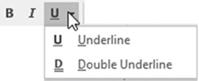
Figure4-2.SelectUnderlineorDoubleUnderline
Changing the Font and
Its Size
It�s important to pick the right font and size not only to make your spreadsheet data stand out but to make
it easy
to read.
Fonts
The font can be changed
by clicking the down arrow for the font and then picking
your selection from a list. See Figure
4-3. The font list shows
how the different fonts look. As you pass your mouse
pointer over the various fonts in the list, Excel
displays the text in the active cell using the font that your mouse
pointer is passing
over. Changing the font affects
the text of all currently selected cells on your worksheet.
90
CHAPTER 4 ■ FORMATTING AND ALIGNING
DATA
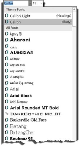
Figure 4-3. Available fonts
There are a lot of fonts
in the list. If you want to jump to a particular font quickly you type the first
letter(s) of the font name in the Font Name Box. For example, if you wanted
to use the font Bell MT you would type the first
three letters Bel (there is only one font that starts with Bel) and then press
Enter.
Font Size
Clicking
the down arrow
for the font size shows
all the available font sizes for the currently selected font. Figure 4-4 shows the top half of the available
font sizes for the Calibri
font.
Figure 4-4. Select font size
91
CHAPTER 4 ■ FORMATTING AND ALIGNING
DATA
Clicking the Increase Font Size button
 �increases the size of the font to the next available font size. Looking
at Figure 4-4 if the current
font size is 11, clicking
the Increase Font Size button will increase
the font size to the next available size, which is 12. If the current
font size is 18, clicking
Increase Font Size will increase
the font size to the next available
size, which is 20.
�increases the size of the font to the next available font size. Looking
at Figure 4-4 if the current
font size is 11, clicking
the Increase Font Size button will increase
the font size to the next available size, which is 12. If the current
font size is 18, clicking
Increase Font Size will increase
the font size to the next available
size, which is 20.
Clicking the Decrease Font Size button
 �does the opposite; it changes the font size to one size less
than the current
size. Looking at Figure 4-4, you can see that if the current
font size is 18, clicking
the Decrease Font Size button will decrease the font size to 16 points. A font size is measured
in points. Each point is approximately 1/72 of an inch.
This exercise covers various ways of selecting fonts and changing font
sizes.
1.
Create a new workbook.
2.
Save the workbook
giving it a name of Chapter
4. Change
the name of the worksheet
from Sheet1 to Font.
3.
Type your name in cell H5 and then press Ctrl + Enter to accept the value.
4.
On the Home tab in the Font group click the down arrow for the Font.
5.
Observe how your name changes
as you move your mouse pointer over the different fonts. Select the font Arial
Narrow if you have it otherwise select another typeface.
6.
Click the down arrow for the font size.
7.
Observe the size of your name as you move your mouse pointer over the different
font sizes. Select
Size 26.
8.
Now, try the Increase and Decrease buttons:
a.
Click the Increase Font Size button. The Font Size changes to 28.
b.
Click the Increase
Font Size button again. The Font Size changes to 36.
c.
Click the Decrease
Font Size button.
The Font Size changes to 28.
d.
Click the Decrease Font Size button. The Font Size Changes to 26.
9.
Double-click cell H5 to put it in edit mode. Drag across the first three letters in
your name to select them.
10.
Click the down arrow for the font. Observe how only the first three letters change as you move
your mouse pointer over the
different fonts.
11.
Type Ti in the Font Name Box to jump to the Times New Roman font. Press Enter.
You should now be familiar
with all of the tools
available on the menu�s Font group. Next,
you will see how you can access
these same tools
from the Font group�s dialog
box launcher.
92
Using the Font Group�s Dialog
Box Launcher
CHAPTER 4 ■ FORMATTING AND ALIGNING
DATA
Clicking the Font group�s dialog box launcher
brings up the Format Cells dialog box with the Font tab active. See Figure 4-5. Here you can specify most of
the options that are also available on the Font group, plus you
can add Effects from one convenient location.
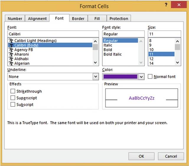
Figure 4-5. Font options
Formatting
with Color
You can change your worksheets from drab to attention grabbing
by adding colors.
You can add colors not only
to make your worksheet more stimulating but also to
�
emphasize
the cells that you think
are important
�
separate different areas of your worksheet
�
make your worksheet easier to read
Be careful
how you use color. Using too many colors or using colors in an incorrect manner such as using dark text
against
a dark background can make your worksheet
confusing and hard to read.
93
CHAPTER 4 ■ FORMATTING AND ALIGNING
DATA
Changing the Font Color
Clicking the Font color button
 �will apply the current color displayed on the icon to the text of your
active cells. You can select a different
color by clicking
its down arrow.
�will apply the current color displayed on the icon to the text of your
active cells. You can select a different
color by clicking
its down arrow.
You can select
any color from the set of Theme
Colors or from the Standard
Colors as shown
in Figure 4-6.
If you want more colors to select from, click the More Colors option.
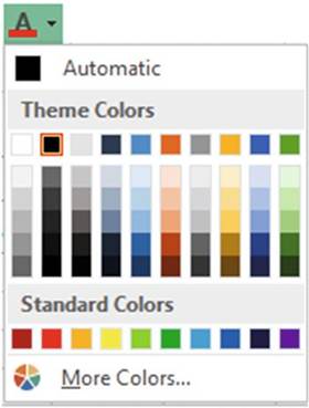
Figure4-6.ThemeandStandardcolors
Clicking the More Colors option brings up the Colors dialog box which has Standard and Custom tabs. The
Standard tab lets you select color from a honeycomb type of grid. The bottom right shows what the font color
is for the current cell. When you select a color from the grid it is displayed in the New area at the bottom
right of the window. See Figure 4-7. This is the color to which the font will be changed if you click the OK
button.
94
CHAPTER 4 ■ FORMATTING AND ALIGNING
DATA
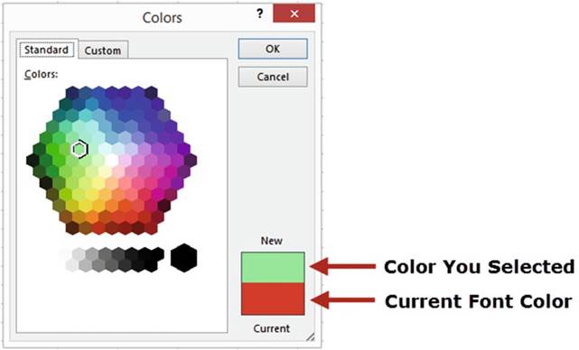
Figure4-7.Selectanewcolorfromthehoneycombofcolors
The Custom
tab shows colors
in vertical bars.
See Figure 4-19. The edge of each vertical
bar blends in with the adjacent color.
You can click
any spot in the color palette that matches the color you need. That color is then displayed in the vertical
bar to the right of the color
palette. Dragging the arrow up or down changes the intensity of the color.
See Figure 4-8.
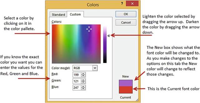
Figure 4-8. Create a custom color
95
CHAPTER 4 ■ FORMATTING AND ALIGNING
DATA
Changing the Cell Background Color
Clicking the Fill Color button
 �will apply the current color displayed on the icon to the background of your active cells. You
can select a different
color by clicking
its down arrow. This will bring up the same options that were available
for the font color.
�will apply the current color displayed on the icon to the background of your active cells. You
can select a different
color by clicking
its down arrow. This will bring up the same options that were available
for the font color.
Clicking the dialog box launcher for the Font group brings up the Format Cells dialog box. The Fill tab in
the Format Cells dialog box has options for creating Fill Effects or a patterned
background. See Figure
4-9.
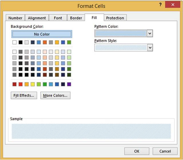
Figure4-9.SelectaFillColor,PatternColor,orPatternStyle
Check Which
Formats Have Been Applied to the Current
Cell
You can tell some of the formats that have been applied to a cell by just clicking the cell and then
observing what is displayed in the Font group on the ribbon.
Looking at Figure
4-10 you can see that the text in cell C1 has
been bolded and italicized. It has an Arial Black
font and has a font size of 16.
■
Note� If all of the text in the cell does not have the same format, you will need to
select those characters
for which you want to reveal their formatting.
96
CHAPTER 4 ■ FORMATTING AND ALIGNING
DATA
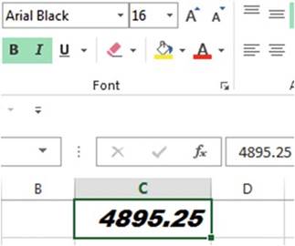
Figure4-10.Selectedtextisboldedanditalicized
The Borders,
Fill Color, and Font Color
options do not reflect the current cell.
They reflect the selection that was made the last time they were used.
This exercise covers changing the font�s color
as well as changing the background color
of a cell. The cell background can be a solid color,
a gradient, or a pattern.
1.
Create a new Worksheet named �Colors.�
2.
Click cell B3. On the Ribbon�s Home tab, in the Font group, click the down arrow for the Fill
Color button
 . Select Black.
3.
Now, type and format some text:
a.
Click the down arrow for the Font Color button
 �and select White.
b.
Type Total Values. Press Ctrl + Enter.
c.
Change the font type to Calibri if it isn�t already.
d.
Click the Increase Font Size button
 �once.
e.
Press Ctrl + B to bold the text.
f.
Widen the column by double-clicking between the column
heads labeled B and C so that all of
the text fits in the cell.
4.
Click cell B4. Click
the down arrow for the Fill Color button. Select
the color �Green, Accent 6, Lighter 80%.� See Figure 4-11.
97
CHAPTER 4 ■ FORMATTING AND ALIGNING
DATA
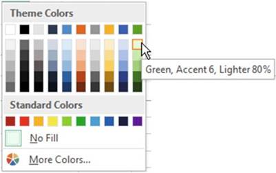
Figure4-11.SelectGreen,Accent6,Lighter80%
5.
Click the down arrow for the Font
Color button. Select Black. Type Total Values in cell B4. Press Ctrl + Enter. Change the font to
Cambria. Change the font size to 14. Click the bold and italics
buttons.
Widen
the column to accommodate the changes.
6.
Click
cell B3 again. You can see what formatting has been applied to the cell. The Bold button is highlighted. The
font shows as Calibri. The font size reflects that you clicked on the Increase Font Size button. Click the
down arrow for the Fill Color
button. The selection box is around the color black. Click the down arrow for the Font Color. The selection
box is around the color white. Click cell B4. See if you can detect what formatting has been applied to it.
Change
Background to a Gradient
1.
Select cells B5:D5. Click the
dialog box launcher
 �for the Font group.
2.
Click the Fill tab.
3.
Click the Fill Effects button.
The Gradient tab is for changing the background to a gradient
color. See Figure
4-12.
4.
Select any color you want for Color 1 and then select another color for
Color 2.
5.
Click each of the shading styles and observe the changes
made to the gradient pattern.
6.
When you have the colors
and style you wish to use, click
the Variant box that
contains the pattern you want to use. The Sample
shows how the background will look using the choices
you have made.
7.
Click the OK button for the Fill Effects dialog
box. Click the OK button
for the Format Cells dialog box.
98
CHAPTER 4 ■ FORMATTING AND ALIGNING
DATA
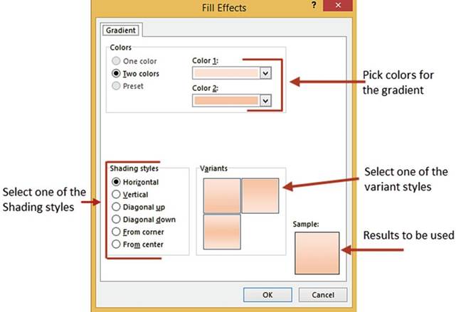
Figure4-12.Changecellbackgroundcolorstoagradient
Change
Background to a Pattern Style
8.
Select cells B7:D8. Click the dialog box launcher for the Font group. Click the Fill tab. Select
a pattern color
of your choice.
Select a pattern
of your choice
from the Pattern
Style drop-down box. Click the OK button.
9.
Click the Save button
 �on the Quick Access Toolbar.
You have learned
how to alter the appearance and size of your text as well as emphasizing it. You can use this knowledge to
draw your user�s eye to the text you want. Your company may have standards
for how your worksheets should look with certain font types and colors. Next, you will see how placing
borders around your cells can also be used to emphasize certain
cells or as a way to show separation of different
areas of your worksheet.
Cell Borders
All cells have grid lines that separate
them. This distinguishes one cell from another. The gridlines can be
removed by selecting the Ribbon�s
View tab and then unchecking Gridlines. See Figure 4-13.
99
CHAPTER 4 ■ FORMATTING AND ALIGNING
DATA
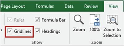
Figure 4-13.Uncheck Gridlines to remove all
gridlines from the worksheet
Figure 4-14 shows the result of removing the Gridlines.
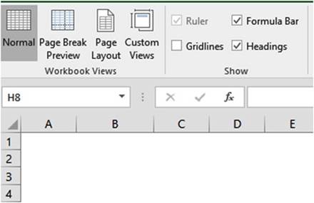
Figure 4-14. No Gridlines
There are times, however,
when you will want to distinguish a particular cell, row, column,
or group of cells. You can do this by using borders.
A border can be just a line at the left, top, right, or bottom of the cell or
range of cells. It can also be a combination of lines or a full box around the cell or range of cells.
Figure 4-15 shows several
different border types.
100
CHAPTER 4 ■ FORMATTING AND ALIGNING
DATA
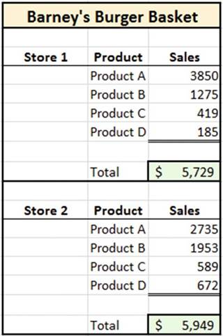
Figure 4-15. Different border types
Clicking the Border button
will apply the border that is currently displayed on the button to your active cells. If you want a
different border style you can click
the down arrow
next to the border and select one of
the options to apply to your selected
cells. See Figure
4-16.
■
Note� Standard accounting practice is to place a single line above and a double
line below a total line.
101
CHAPTER 4 ■ FORMATTING AND ALIGNING
DATA
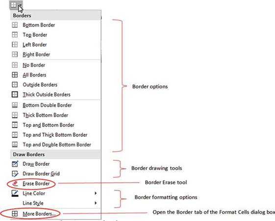
Figure 4-16. Border options and tools
■
Note� You can erase a portion
of a border by using
the Erase Border
tool. The mouse
pointer will display
as an eraser when using
the Erase Border
tool.
Drawing Borders
You can even draw your borders by using either the Draw Border or Draw Border Grid tool. Your mouse pointer
will display as a pencil when using one of the drawing
border tools. The border will be drawn in the current line style.
The Draw Border tool draws a full outside
border around the cells you drag across.
See Figure 4-17.
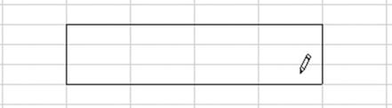
Figure 4-17. Draw Border tool
102
CHAPTER 4 ■ FORMATTING AND ALIGNING
DATA
The Draw Border Grid tool places a full border around each cell. See Figure 4-18.

Figure 4-18. Draws Border Grid tool
In this exercise you will use various methods
of creating borders as well changing border width, style, and color.
Add
Borders Using the Border Button
1.
Create a new worksheet named
�Borders.�
2.
Select cells B2:C2
3.
On the Ribbon�s Home tab,
in the Font group, click the
down arrow for the Borders button.
4.
Click Top and Double Bottom Border. Click another cell so that you can see the results.
Draw
Borders
1.
Click the down arrow for the Borders button in the Font group.
2.
Click Draw Border. The mouse pointer should turn into a
pencil.
3.
Draw a border around cells B4 to B8. Notice that the Border button�s icon has changed to a pencil
to reflect your selection.
4.
Click the down arrow for the Border
button.
Notice that there is now a shadow around the Draw Border button to indicate
that the tool is currently active. Also, notice
that the Line Color button has a colored line on it. This indicates
the color that is currently
being used.
When you change the Line Color or the Line Style you are making changes to the currently
active tool which is currently
the Draw Border tool.
5.
Click Line Color.
Select the green
color from the Standard Colors.
See Figure 4-19.
103
CHAPTER 4 ■ FORMATTING AND ALIGNING
DATA
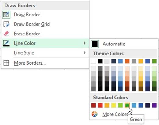
Figure4-19.Changetheborder�slinecolor
6.
Draw a border around cells B10:C13. The
border should appear in green.
7.
Click the down arrow for the Border button. Click the Draw Border button to deselect
it.
8.
Click the down arrow for the Border button. Click Line
Style. Select the double line.
See Figure 4-20.
104
CHAPTER 4 ■ FORMATTING AND ALIGNING
DATA
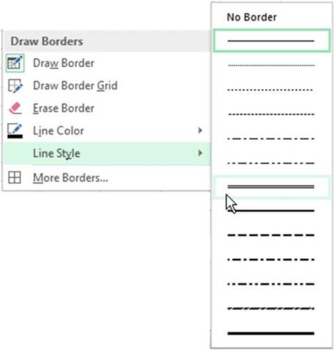
Figure4-20.Changetheborder�slinestyle
If neither the Draw Border
tool nor the Draw Border
Grid tool is active when you select
the Line Color
or Line Style,
Excel will automatically turn on the Draw Border
tool.
9.
Draw a border around cells B15:C19. See Figure 4-21.
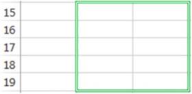
Figure4-21.DrawaborderaroundthecellrangeB15:C19
10.
Press the Escape key to turn off the Draw Border mode.
105
CHAPTER 4 ■ FORMATTING AND ALIGNING
DATA
Draw a
Border Grid
1.
Click the down arrow for the Border
button. Notice that the Draw Border tool is no longer active.
Pressing the Escape
key made it inactive.
2.
Click Draw Border Grid
3.
Draw a border around cells
E3:F7. The border
should appear as a green
double line since
these are the last options
you selected.
The Border button icon has changed to reflect
that the Draw Borders Grid tool is currently
active. See Figure 4-22.
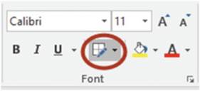
Figure 4-22.Border button reflects that the Draw
Borders Grid tool is active
4.
Click the down arrow for the Border button. Notice
that the Draw Border Grid tool is currently active.
Select Line Color.
Select the Red color from the Standard
Colors.
5.
Draw a border around cells E10:F12 and press the Escape key
6.
Select cells I2:J6
7.
Click the down arrow for the Border button. Select
Top and Thick Bottom Border. Click
another cell to see the result. (Notice
that the lines now appear in red because this is the last line color that you used)
Create a
Border Using the Format Cells Dialog Box
1.
Click cell I8
2.
Click the down arrow for the Border button. Select More Borders
3.
Create a border:
a.
Select the first solid line in the second column of the Style group.
b.
Select Automatic for the color
c.
Click Outline in the Presets area. The Preview
box in the Border area displays what the cell will look like. See Figure 4-23.
106
CHAPTER 4 ■ FORMATTING AND ALIGNING
DATA
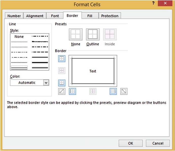
Figure 4-23.Preview Box in Border area displays
what the border will look like
4.
The Inside option
in the Presets area is grayed out because there is only one active
cell and that is cell I8. Click
None in the Presets
area. This removes
all borders from the Preview
box.
5.
Click the top border button
in the Border area. A top border
is displayed in the Text box. See Figure 4-24.
107
CHAPTER 4 ■ FORMATTING AND ALIGNING
DATA
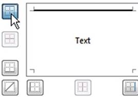
Figure4-24.Topborderbuttoncreatesatopborder
6.
The Border buttons
work like toggle switches. Clicking
a Border button puts that border in the cell. Clicking the Border button again will remove that border.
Click the top Border button to remove the border from the cell.
7.
Click the left Border button and then the right Border button. See Figure 4-25.
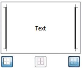
Figure 4-25.Left and right Border buttons create
left and right borders
8.
Click the OK button. Click
another cell so that you can see the results.
Cell I8 should now have a left and right border.
9.
Select cells E15:F20.
10.
Click the down arrow for the Border
button. Select More Borders. Because multiple cells
are selected, the Inside button
in the Presets area and all the borders in the Border area are available.
11.
Click the Vertical Click Inside button
 .
.
12.
Click the None button in the
Presets area to clear the Preview area.
13.
Select the first solid line in the second column of the Style group.
108
CHAPTER 4 ■ FORMATTING AND ALIGNING
DATA
14.
Select Red for the color.
15.
Click the Outline button
in the Presets area. This activates
the top, bottom, left, and right Border buttons.
16.
Select Green for the color.
17.
Click the horizontal inside button
 . See Figure 4-26.
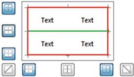
Figure
4-26.ThehorizontalBorderbuttoncreateshorizontalborder
18.
Click the OK button.
Erase
Borders
1.
Click the down arrow for the Border
button.
2.
Select Erase Border. The mouse pointer
becomes an eraser
 . Clicking a border line with the tip of the eraser
will remove that border line.
. Clicking a border line with the tip of the eraser
will remove that border line.
3.
Erase the first, third, and fifth horizontal green lines. Since
the horizontal lines
are two cells wide, you will need to click
the horizontal line for each cell. You will probably
find it easier
just to hold down the left mouse
button and drag across the horizontal line.
See Figure 4-27. If you erase
too much, just click the Undo button
 �or press
Ctrl + Z and try again.
�or press
Ctrl + Z and try again.
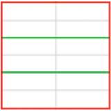
Figure 4-27.Erased
the first, third,
and fifth inside
border horizontal lines
109
CHAPTER 4 ■ FORMATTING AND ALIGNING
DATA
4.
Press the Escape key. This
turns off the Eraser tool.
5.
Click the Save button
 �on the Quick Access Toolbar.
Formatting Numeric Data Using the Number Group
You have seen how Excel
makes assumptions based
on the data you entered
as to how that data should be formatted and aligned in the cell,
such as right-aligning numeric data. If you want to change
that formatting, you will need to use one of Excel�s
many formatting features
which are located
in the Number group on the
Home tab. See Figure 4-28. Table 4-1 provides a description for each of the options
in the Number group.
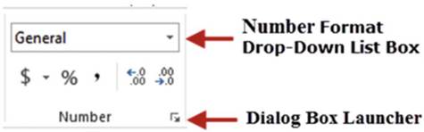
Figure4-28.Ribbon�sNumbergroupontheHometab
Table4-1.DescriptionforEachOptionintheNumberGroup

Buttons on Number Group Description

The Number Format
drop-down list provides
various defaults for numeric,
date, and time values. See Figure 4-26.

Clicking
the dollar sign portion of the button
formats the current
cell in the Accounting format (dollar signs,
commas, and two decimal positions). If you want to use a different currency
such as pounds
or euros you can click
the down arrow to the right
of the
 button.

Multiplies
the value in the cell by 100 and adds a % sign to the end of the value.

Adds commas to a value. If the value doesn�t already contain a decimal it
will add .00 to the value.

The first button (Increase Decimal)
increases the number of decimal
positions in the cell by one each time you click it. The second button (Decrease
Decimal) decreases the number of decimal positions
in the cell by one each time you click
it.

Dialog box launcher brings up the Format Cells dialog box with the Number tab selected.
110
CHAPTER 4 ■ FORMATTING AND ALIGNING
DATA
Using
Default Formats
Let�s
say that the active cell currently has a value of 3859.27.
Clicking the drop-down arrow of the Number Format drop-down list displays a list of default formats (see
Figure 4-29). Clicking an option in this list formats the current value as shown below each format label.
What you see is what you get. There are no options to select.
For example, if you were to click
the Fraction option,
the format of the current
cell would change
and the result would be 3859 �.
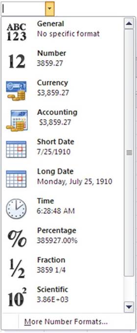
Figure4-29.Defaultformatsfordifferentdatatypes
111
CHAPTER 4 ■ FORMATTING AND ALIGNING
DATA
Accounting
and Currency Formats
The Accounting format
is a special monetary format
that displays values
with a dollar sign, commas,
and two decimal positions. The Accounting format
lines up the dollar signs
and decimal points
in a column. See
Figure 4-30. The dollar sign is always placed in the left-most position
in the cell. Depending upon the width of
the cell and the value you have in it there could be many spaces between
the dollar sign and the value itself.
The Currency format is similar
to the Accounting format. It also adds dollar signs,
commas, and two decimal positions to values.
The difference is that the Currency format
uses a floating dollar sign and the Accounting format
uses a fixed dollar sign.
The floating dollar
sign doesn�t align
the dollar, signs;
instead, it places the dollar
sign to the immediate left of the value.
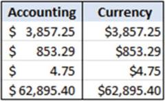
Figure4-30.DifferencebetweenAccountingandCurrencyformats
Formatting
Monetary Values
The
 button in the Number group performs the exact same formatting as selecting the Accounting format
from the Number Format drop-down list. If you want to display the value in a different
format or if you want to
use a different currency such as pounds or euros you can click the down arrow to the right of the
button. See Figure
4-31.
button in the Number group performs the exact same formatting as selecting the Accounting format
from the Number Format drop-down list. If you want to display the value in a different
format or if you want to
use a different currency such as pounds or euros you can click the down arrow to the right of the
button. See Figure
4-31.
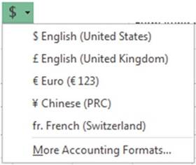
Figure4-31.Formattedmonetaryvalues
If you want to use something other than two decimal positions
or you want to use a currency
other than those shown in the drop-down box, you can select the last option
More Accounting Formats. Selecting this option is one of the many ways of opening the Format Cells
dialog box.
112
CHAPTER 4 ■ FORMATTING AND ALIGNING
DATA
From here you can select one of the many different
currency options available
in the Symbol drop- down list. See Figure 4-32.
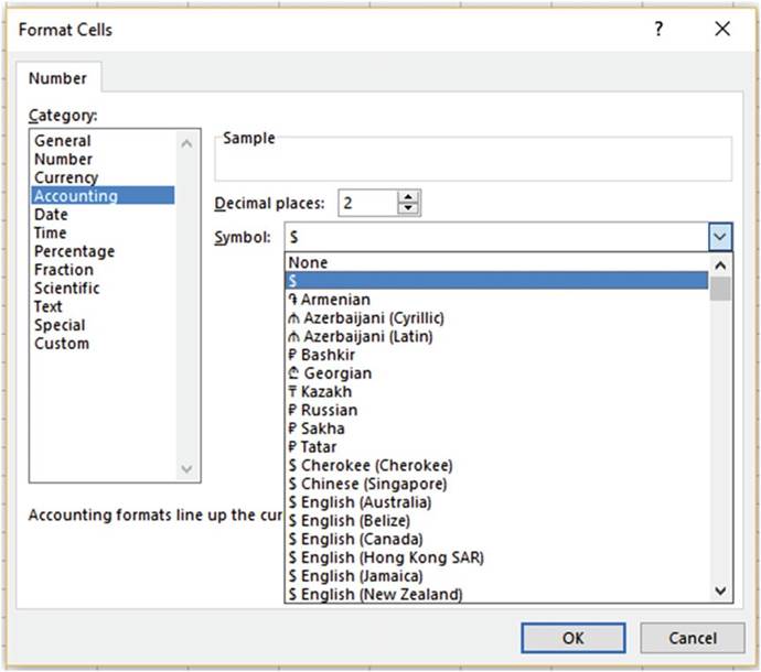
Figure4-32.Accountingoptionsfordecimalplacesandmonetarysymbol
Converting
Values to Percent Style
The Percent Style
 �button multiplies the values in your selected
cells by 100 and places
the % after the number. The value .25 would be formatted as 25%. The % button
rounds the value
and then removes
any decimal positions as shown in Figure 4-33.
�button multiplies the values in your selected
cells by 100 and places
the % after the number. The value .25 would be formatted as 25%. The % button
rounds the value
and then removes
any decimal positions as shown in Figure 4-33.
113
CHAPTER 4 ■ FORMATTING AND ALIGNING
DATA
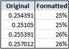
Figure4-33.Formattedusingpercentstyle
If you want to use a percentage format that displays
two decimal positions, then click the Number
Format drop-down arrow and select % (percentage) See Figure 4-34.
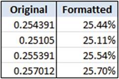
Figure 4-34. Formatted with % option
Converting Values to
Comma Style
The Comma Style
 button places
comma separators in the values
for the cells
you have selected. The value 3857495.25 would
be formatted as 3,857,495.25
button places
comma separators in the values
for the cells
you have selected. The value 3857495.25 would
be formatted as 3,857,495.25
Changing the Number of
Decimal Places
The
 �Increase Decimal button increases the number of decimal positions
by one for each time you click it.
The icon shows a single decimal place changing to two decimal
places.
�Increase Decimal button increases the number of decimal positions
by one for each time you click it.
The icon shows a single decimal place changing to two decimal
places.
The
 �Decrease Decimal button decreases the number
of decimal places by one each time you click
�Decrease Decimal button decreases the number
of decimal places by one each time you click
it. The icon shows two decimal places
changing to one decimal place.
Accessing the Format Cell Dialog Box
If you want to use more options
when formatting a number, then using the Number tab in the Format Cells dialog box is the way to go. Using
the Number tab in the Format Cells dialog box you can do such things as format fractions, dates, times, and
other formatting that you can�t do in the other sections. What options
appear on the right side of the window depends
upon the category
selected. See Figure 4-35.
114
CHAPTER 4 ■ FORMATTING AND ALIGNING
DATA
The Format Cells dialog box can be accessed
from the Number group by using any of the following
methods:
�
Click the Dialog Box Launcher
�
Click the drop-down arrow
for the Number Format drop-down box then select More Number Formats.
�
Click the down arrow to the right of the $ button and then select MoreAccounting
Formats
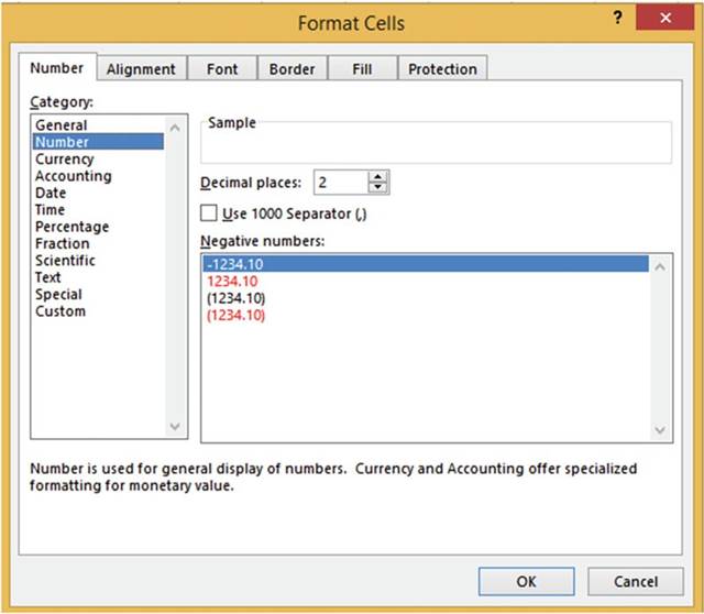
Figure4-35.FormatCellsdialogboxwithNumberformattingselected
In this exercise,
you use various numeric data formats. If you have closed your workbook from the last practice you can reopen
the Chapter
4 workbook.
1.
Create a new worksheet named �NumberGroup.�
115
CHAPTER 4 ■ FORMATTING AND ALIGNING
DATA
2.
Type 1275.85 in cell A1 but don�t press Enter. Click
the Enter button
in the formula bar
 . Clicking the Enter button
accepts the value you entered
and leaves the current cell as the active cell.
Once the value has been accepted the check and delete buttons
are grayed out on the formula bar.
. Clicking the Enter button
accepts the value you entered
and leaves the current cell as the active cell.
Once the value has been accepted the check and delete buttons
are grayed out on the formula bar.
3.
On the Home tab, in the Number
group, click the down arrow for the Number Format drop-down box
 . Notice that every option
on the drop-down box shows how the value in A1 will appear if you click that particular format.
. Notice that every option
on the drop-down box shows how the value in A1 will appear if you click that particular format.
■
Note� Excel�s calendar starts
with the date January 1, 1900. Notice
that the Short
Date and Long Date formats
show the date as June 28, 1903.
This date is displayed because
the integer portion
of the value that you entered
in cell A1 is 1275 and the date June 23, 1903 is
1,275 days past January 1, 1900.
4.
Click the Currency format.
5.
Change the width of Column A to approximately 13.43
6.
Type 3427.35in cell A2 but don�t press Enter. Click the Enter button in the formula bar.
7.
Click the Accounting Number Format button
 in the Number group. Notice the difference between the Currency
format in cell A1 and the Accounting format in cell A2. The $ appears
in the left-most position of the cell when using the Accounting format. The Accounting format also leaves
one blank space to the right of the last digit.
in the Number group. Notice the difference between the Currency
format in cell A1 and the Accounting format in cell A2. The $ appears
in the left-most position of the cell when using the Accounting format. The Accounting format also leaves
one blank space to the right of the last digit.
8.
Type .85 in cell A3. Press Ctrl + Enter.
Click the % button in the Number group. The value should display as 85%.
9.
Enter 1385197 in cell A4. Press Ctrl + Enter.
Click the Comma Style button
 �in the Number group. The value displays
as 1,385,197.00.
�in the Number group. The value displays
as 1,385,197.00.
10.
Click the Decrease
Decimal button
 . One of the decimal
positions is removed.
Click the Decrease
Decimal button a second time. The second decimal position
is removed. Click
the Increase Decimal
button
. One of the decimal
positions is removed.
Click the Decrease
Decimal button a second time. The second decimal position
is removed. Click
the Increase Decimal
button
 �twice to change the value back to having two decimal
positions.
�twice to change the value back to having two decimal
positions.
11.
Enter -385 in cell C1. Press Ctrl + Enter.
Click the down arrow for the Number Format drop-down
box. Notice that the Currency
format displays the value as
-$385.00 but the Accounting format displays it as ($385.00). In Accounting
negative numbers are displayed in parentheses.
■
Note� Notice that the Scientific format displays the value as -3.85+E02. The
Scientific format when dealing with whole numbers puts the decimal after the left-most digit, rounds the
number to two decimal
positions, and displays the rest as an exponent.
116
CHAPTER 4 ■ FORMATTING AND ALIGNING
DATA
12.
Click Accounting to change the format
in cell C1.
13.
Enter
3.25 in cell C2. Press Ctrl + Enter.
Click the down arrow for the Number
Format drop-down box. Click Fraction. The Fraction format
converts the decimal
portion of a number to a fraction. The fraction portion
.25 is changed to 1/4.
14.
Enter 5/15/2012 into cell C3. Press Ctrl + Enter.
Click the dialog
box launcher on the Number
group, shown in Figure 4-36, to bring up the Format
Cells dialog box. See Figure
4-37.
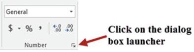
Figure 4-36. Number group
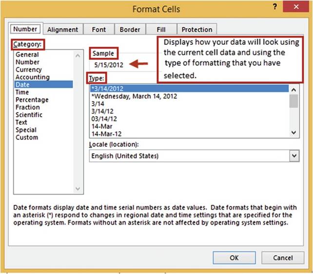
Figure4-37.FormatCellsdialogboxwithNumbertabselected
117
CHAPTER 4 ■ FORMATTING AND ALIGNING
DATA
Excel recognizes the value as a date and so it opens the Format
Cells dialog box with the Date category
selected. After the category has been selected
you will need to select
how you want your data to appear
from the Type area. The Sample area of the window displays
how the data in the current cell will appear
using the option
you selected from the Type area. If you have a range
of cells selected
on the worksheet it will show how the first
cell in that range will appear.
15.
Click Number in the Category
area. The Number
category has options
for entering the number of decimal positions, for using a comma, and for letting
you select how you want to display
negative numbers.
16.
Click each of the other categories to familiarize yourself
with the different options for formatting your data.
17.
Click
the Date Category
again.
18.
In the Type area, Select
*Wednesday, March 14, 2012. The Sample area shows how this change
will display the current cell.
19.
Click the OK button.
20.
Cell C3 may display as a number of # signs. What does this mean? That�s
right, the column
isn�t wide enough.
Widen the column to see your results.
21.
Click the Save button
 �on the Quick Access Toolbar.
You have learned how to use the tools
from the Ribbon�s
Number group to format numeric
data.
Formatting
the data is necessary so that the user can interpret the data the way it was meant
to be, such as making sure the user knows
a number is a percentage and not just a numeric
value. Next, you will learn
how to align data within
a cell.
Aligning Data Using the Alignment Group
The Alignment group is located
on the Home Tab. See Figure 4-38. It contains options
for aligning your text
vertically and horizontally, rotating text, increasing and decreasing indenting, word wrap, and merging
cells. Table 4-2 provides a description for each option in the Alignment group.
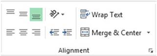
Figure4-38.AlignmentgroupontheHometab
118
CHAPTER 4 ■ FORMATTING AND ALIGNING
DATA
Table4-2.DescriptionsofAlignmentButtons

Buttons������ Description

VerticalAlignment�The Top-, Middle-, and Bottom-Align buttons are for aligning your text to the
top of the cell, the middle of the cell, and the bottom of the cell in that order.

Orientation�Clicking this button brings
up options for selecting the angle and direction of the text within a cell.

Wrap Text�Used for wrapping
your data across
multiple lines within
a cell

HorizontalAlignment�The Left-, Center-, and Right-Align buttons are for aligning your text to
the left side of a cell, to the middle of a cell, and to the right side of a cell in that order.

Indentation�The Decrease
Indent button (left)
is for decreasing the amount
of indentation in a cell.
The Increase Indent
button (right) is used for increasing the amount of indentation in a cell.
 ��
Merge
& Center�This button provides options for merging
cells, merging and centering cells,
and unmerging cells.
��
Merge
& Center�This button provides options for merging
cells, merging and centering cells,
and unmerging cells.
Fitting More Text into a Cell
Excel provides three
options for fitting
more data into a cell. Text Wrapping�Text automatically wraps to the next line
Shrink to Fit�Shrinks the size of the cells contents so that they fit within the cell Merge Cells�Merges
multiple cells into a single cell
Text Wrapping
If your text doesn�t fit within a cell you might want to break
up the text on to multiple lines.
Turning Word Wrap on will format the cell so that the text wraps
automatically. You can turn word wrap on by selecting the cell(s) you want to automatically word wrap and
then clicking
the Home tab in the Ribbon. In the Alignment group, click the Wrap Text button. You can also force a line
break
to occur wherever
you want by pressing ALT + Enter.
■
Note� When word wrap is turned on, data
in the cell wraps to fit the column width. When
you change the column width, data
wrapping adjusts automatically.
Figure 4-39 shows a before and after example of using Wrap Text
119
CHAPTER 4 ■ FORMATTING AND ALIGNING
DATA
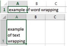
Figure 4-39.The upper part of the image shows
text before using Wrap Text,
and the lower part shows
text after Wrap text has been applied
Shrinking to Fit
Turning on the Shrink to fit option
will shrink the cell�s contents
so that they will fit within the size of the cell. Figure 4-40 shows a before
and after example.
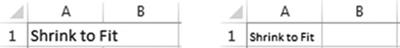
Figure 4-40.The image on the left shows text before using
Shrink to fit, and the one on the right shows it after Shrink
to fit has been applied
If you enter very much text,
it may become too small
to see unless you expand
the width of the column. The Shrink to fit option is located on the Alignment
tab of the Format Cells dialog box. See Figure
4-41. There are several ways to open this tab. One way is to click the dialog box launcher of the Alignment
group and then select the Alignment tab.
120
CHAPTER 4 ■ FORMATTING AND ALIGNING
DATA
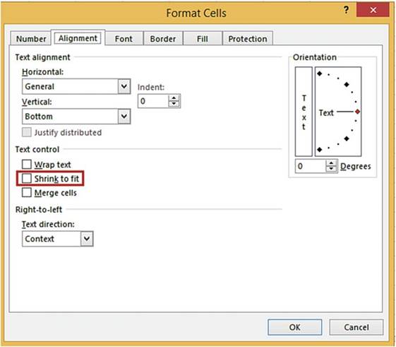
Figure4-41.FormatCellsdialogboxwithAlignmenttabselected
The Shrink to fit option can be turned on or off by selecting
or clearing the Shrink to fit check box.
Notice that there
are also options
here for turning
on Wrap text and Merge
cells.
Merging and Unmerging Cells
You can join multiple cells
to make one larger cell by using
one of the three different options for merging
cells.
�
Merge & Center
�
Merge Across
�
Merge Cells
The Merge
& Center option
merges the selected cells and then centers the data horizontally in the new expanded cell. The Merge &
Center
button is located on the Home Tab |
Alignment group.
You can improve the look of your spreadsheet by making your heading centered
across the width
of your worksheet. In Figure
4-42, the heading
has been entered
into cell A1. The heading
would look better
if it were centered
across columns A through F.
121
CHAPTER 4 ■ FORMATTING AND ALIGNING
DATA
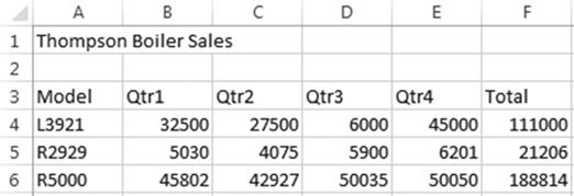
Figure4-42.Headingbeforebeingcentered
To center
the heading across
the cells, you select the cells and select the Merge &
Center option. When you
merge cells A1, B1, C1, D1, E1, and F1, you end up with one cell that takes
up the space of all six cells.
See Figure 4-43. The single cell will have an address
of A1.
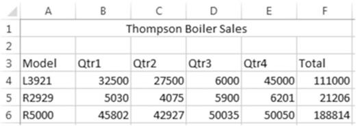
Figure4-43.Cellsmergedandtheheadingcentered
The Merge & Center command lets you merge cells that are not only adjacent
horizontally but vertically as well. Even though you can merge cells that are vertically adjacent, the Merge
& Center command is usually used for creating
labels that expand multiple columns
or for spanning a heading
over a report.
All the Merge options
can be accessed by clicking
the down arrow to the right of the Merge & Center button. See Figure 4-44.
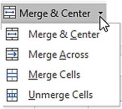
Figure 4-44. Merge options
122
CHAPTER 4 ■ FORMATTING AND ALIGNING
DATA
The other three options do the following:
�
The Merge Across
option can only merge cells
that are horizontally adjacent. It does not
center the text.
�
The Merge Cells option can merge cells that are horizontally or vertically adjacent.
Like the Merge Across option it does not center the text.
�
You can unmerge cells
by selecting the cells you want to unmerge and then clicking the Unmerge Cells option.
Aligning
and Indenting Text in a Cell
Excel provides options for setting the
alignment for data in a cell (see Table 4-3) and for increasing or decreasing indentation in a cell
(see Table 4-4).
Table4-3.VerticalandHorizontalAlignment

Buttons���� Description

VerticalAlignment�These buttons are for aligning your text to the top of the cell, the middle
of the cell and the bottom of the cell in that order. Excel bottom aligns cell data by default.

HorizontalAlignment�These buttons are for aligning your text to the left side of a cell, to the
middle of a cell, and to the right side of a cell in that order.
Table4-4.IncreasingandDecreasingIndentationofTextinaCell
Buttons���� Description

Decrease Indent�used to decrease
the amount of indentation in the cell.

Increase Indent�used to increase
the amount of indentation in the cell.
Align
Text Vertically and Horizontally
There are other
options on the Alignment tab of the Format Cells
dialog box for Horizontal and Vertical alignment.
See Figure 4-45. Some of these
are the same as those
that appear on the Alignment group of the Home Tab, but here you have additional options
such as the ability to set the amount of indention for the
Left, Right, and Distributed horizontal alignments by using
the Indent numerical text box.
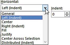
Figure 4-45. Alignment options
123
CHAPTER 4 ■ FORMATTING AND ALIGNING
DATA
The Distributed horizontal alignment uses an
equal amount of indention on both sides of the cell text.
Therefore
if you enter 3 for the Indent
the cell will have three
blanks spaces to the left and to the right
of whatever is entered
in the cell.
The Justify
horizontal alignment option is only useful when you are entering multiple
lines of text in a cell. Excel justifies each line except the last line by adjusting the space
between
words so that the text spreads completely from the left to the right borders
of the cell. See Figure 4-46.

Figure 4-46. Justify alignment
Rotating
Text
Clicking
the Orientation button
(Figure 4-47) displays a list of options for rotating your text. The first five default options
are self-explanatory. If you want to specify
another particular orientation, select the last option Format Cell Alignment. This option
displays the Alignment tab on the Format Cells dialog box.
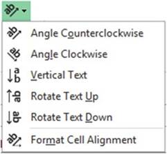
Figure 4-47. Orientation options
The Orientation section on the Alignment tab of the Format Cells dialog box is for setting the angle of your
text.
See Figure 4-48.
124
CHAPTER 4 ■ FORMATTING AND ALIGNING
DATA
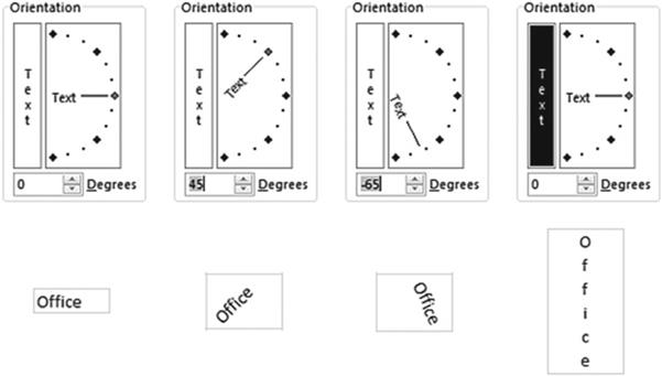
Figure4-48.Optionsforsettingtheangleofyourtext
You can set the angle that your text will be displayed by dragging the line up or down or by setting the
degrees. If you enter the number of degrees
Excel automatically adjusts
the line and vice versa. Moving the line up from 0 degrees makes the text display from bottom to top. Moving
the line down from 0 degrees
makes the text display from top to bottom. If you are entering the degrees and you want your text to display
top to bottom, you will need to enter a negative value. Clicking the Text button on the left side of the
Orientation box puts the text in a completely vertical format.
■
NoteWhen you rotate
text, the size of the cell
automatically adjusts to fit the rotated text.
For this exercise
we will create the worksheet
shown in Figure
4-49. The worksheet
shows information for students attending
the Office Integration and Financial Management classes at Wonderland University.
125
CHAPTER 4 ■ FORMATTING AND ALIGNING
DATA
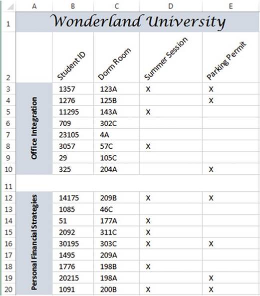
Figure4-49.Worksheetyouwillcreate
1.
If you have closed your workbook from the last practice, you can open the Chapter
4 workbook and then create
a new worksheet named �Align.�
2.
Type Wonderland University in cell A1. Click the Enter button on the formula bar.
3.
Select cells A1:E1. Click the Merge & Center button
4.
Select the Lucida Calligraphy font. Change
the font size to 18.
5.
Type the column head Student ID in cell B2 and then press the Tab key.
6.
Type the rest of the Column Heads in row 2.
We want to place the column headings at a
45-degree angle. Before we do that we
need to widen the columns.
126
CHAPTER 4 ■ FORMATTING AND ALIGNING
DATA
■
Note� If you do not widen the columns you will end up with multiple column heads in
the same column as shown below.

7.
Drag across column
heads B through E. On the ribbon�s
Home tab in the Cells group click the Format
button. Select Autofit Column Width.
8.
Select cells B2:E2.
9.
In the alignment
group click the Orientation button
 �and then select Angle Counterclockwise. Each of the column heads should now appear at a
45-degree
angle in their separate columns.
�and then select Angle Counterclockwise. Each of the column heads should now appear at a
45-degree
angle in their separate columns.
10.
Type 1357 in
cell B3 and then press the Tab key. Since the value is a number it should
appear right-justified in the cell.
11.
Type 123A in cell C3 and then press the Tab key. Since
the value contains
a letter it is considered a text or string value and is left-justified in the cell.
12.
Type a capital X in cell D3 and
then press the Tab key. X is text so it is left justified.
13.
Type a capital X in cell E3 and
then press the Enter key.
14.
Continue typing the rest of the data in cells B4:E10.
15.
Select cell range A3:A10 by dragging across
the cells or by typing A3:A10 in the Name box and then pressing
Enter. Click the Merge &
Center button
16.
Type Office Integration. Don�t worry about how the text looks at the moment.
Press Ctrl + Enter.
17.
Click the Orientation button
�and then select Rotate Text Up
18.
Click the Bold button
 �or press Ctrl + B.
19.
Click the Middle Align button
 �in the top row of
the Alignment group.
�in the top row of
the Alignment group.
20.
Next we want to create a defining space between the two classes:
a.
Select cells A11:E11. Click the Merge & Center button
b.
Increase the height of row 11 to approximately 22.5 by
clicking between row heads 11 and 12 and then dragging down.
21.
Type the data in cells B12:E20.
22.
Select cell range A12:A20 by dragging across
the cells or by typing
A12:A20 in the Name box and then pressing Enter.
127
CHAPTER 4 ■ FORMATTING AND ALIGNING
DATA
23.
Click
the Merge & Center button.
24.
Type Personal Financial Strategies. Don�t worry about how the text looks at the moment.
Click the Enter button on the formula
bar.
25.
Click
the Orientation button
`
 and then select
Rotate Text Up.
and then select
Rotate Text Up.
26.
Click
the Bold button
�or press Ctrl + B.
27.
Click the Middle Align
button
 . The
text extends slightly beyond its border. We will use Shrink to fit so that it fits completely in the
cell.
. The
text extends slightly beyond its border. We will use Shrink to fit so that it fits completely in the
cell.
28.
Click the dialog box launcher on the Alignment group. In the Text Control
area click
Shrink to fit. Click the OK button.
29.
Click cell A1, hold down the Ctrl key, and then click cells A3 and A12. Click the down arrow for
the Fill Color button located
in the Font group. Select the Blue-Gray, Text 2, Lighter
80% color. See Figure 4-50.
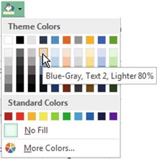
Figure 4-50. Color selections
30.
We could improve the look of our spreadsheet by having the
data appear just a little to the right of the left cell border:
a.
Select cells B3:E10. Click the Increase Indent button
 �in the Alignment group.
b.
Select cells B12:E20. Click the Increase Indent button
 .
.
31.
Type your full name in cell B22 and then press Ctrl + Enter.
Right-click cell B22. Select Format
Cells. On the Alignment tab, check Shrink to Fit. Click the OK button. Your name should
fit completely within
the cell.
32.
Right-click cell B22. Select Format
Cells. On the Alignment tab, check Wrap Text. Click the OK button.
128
CHAPTER 4 ■ FORMATTING AND ALIGNING
DATA
33.
Type your last name in cell C23 and then press Ctrl + Enter. Right-click cell C23. Select
Format Cells. Click the vertical
word Text on the left side of the Orientation box. Click the OK button.
34.
With cell C23 still selected, click the following buttons on the Alignment group: click
the Align Left button, then click the Align Right button, and
then the Center button.
35.
Click the Save button
 �on the Quick Access Toolbar.
You have learned
how to use the commands
from the Ribbon�s
Alignment group to align data both horizontally and vertically within a cell as well as rotating
cell data. You practiced Merging
Cells so that data can occupy more than one cell. The Word Wrap and Shrink to fit features allowed
you to place more text in a cell. Next, you will see how you can copy all the formatting that you applied
to a cell to other cells.
Using Format Painter to Copy Formatting
The Format Painter
can be used for copying
all the formatting in one cell to other cells. The Format Painter
button has an icon of a paintbrush. It appears on the Clipboard
group of the Home tab. See Figure
4-51.
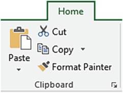
Figure 4-51. Clipboard group
The Format
Painter not only speeds up the process
of applying the same formatting to other cells
but also makes it easy to give your workbook a consistent look.
Single-clicking the Format Painter
button allows you to copy the formatting of a selected
cell to a single range of cells
and then it is automatically turned off. Double-clicking the Format Painter
button keeps the button turned on so you can keep applying
the formatting to as many cell ranges as you want until you click the button again to turn it off.
This exercise takes you through the process
of copying formatting that has been applied to one cell to other cells.
1.
If you have closed your workbook from the last practice you
can open the Chapter 4 workbook, then
create a new worksheet named �Format.�
2.
Click cell A1. Type Copy formatting and then press
Ctrl + Enter.
3.
Widen Column A so that all the
text appears in the cell.
129
CHAPTER 4 ■ FORMATTING AND ALIGNING
DATA
4.
Type the word Data in cells B2 and C3. Use the AutoFill
Handle on cell C3 and drag down to cell C5. Let go of your left mouse button.
Drag the AutoFill
Handle to cell E5. See Figure 4-52.
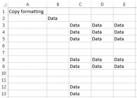
Figure 4-52. Result of using AutoFill
5.
Type the word Data in C8. Use the AutoFill Handle to drag to E9. Type Data in C12
and use the AutoFill Handle to drag to C13.
6.
Format cell A1 by selecting the following options
from the Font group: Bold,
Italic, and Underline; change the text color to red.
7.
Click the Center button on the Alignment tab.
8.
With cell A1 selected, click
the Format Painter
button. The Format
Painter button should now be highlighted. The mouse pointer
changes to a block plus sign with a paintbrush. See Figure 4-53.
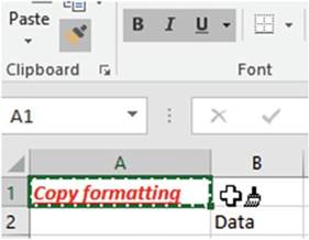
Figure4-53.FormatPainterselectedwithcellA1active
130
CHAPTER 4 ■ FORMATTING AND ALIGNING
DATA
9.
Click cell B2. Cell B2 takes on all the formatting that you applied
to cell A1. The Format
Painter button should no longer be highlighted. Your mouse pointer
should return to
 .
.
10.
Select cell A1. This time double-click the Format Painter
button. The mouse
pointer will stay as
 �and you can keep copying
the formatting until
you turn off the format
painter.
�and you can keep copying
the formatting until
you turn off the format
painter.
11.
Drag across cells C3:E9. Those
cells now have the same formatting as cell A1.
12.
Drag across cells
C12 and C13. Those cells
now have the same formatting as cell A1. See Figure
4-54.
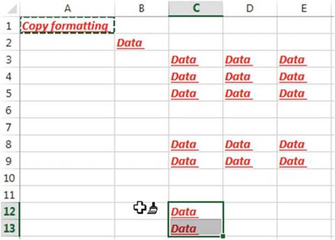
Figure4-54.ResultofapplyingtheFormatPainter
13.
Click the Format Painter button again to turn it off. Your mouse pointer should return to

14.
Since you dragged across cell C6 when you copied the
formatting, if you type something in this cell it should take on
the same formatting as cell A1. Type horse in cell C6.
15.
If you want to clear the formatting from a cell(s),
you can clear just the formatting and leave the data in the cell. Drag across cells C6:E8.
Click the down arrow for the Clear button located
in the Editing group. Click Clear Formats.
See Figure 4-55.
131
CHAPTER 4 ■ FORMATTING AND ALIGNING
DATA
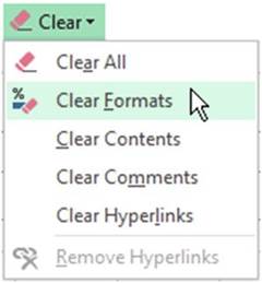
Figure 4-55. Clear options
16.
Click the Save button
 �on the Quick Access Toolbar.
You have been using
commands from the Ribbon. Most of these
commands are more quickly accessible from a mini-toolbar or the context
menu which brings
up commands that relate to what you are currently working on.
Using the Mini-Toolbars and the Context Menu
You have gone through Excel�s
tools for formatting both numeric and text data.
You will no doubt be using
these tools often; therefore Microsoft gives you quick
access to them via the mini-toolbars. There
are two different size mini-toolbars.
If you select any text within
a cell you will see the smaller
of the two mini-toolbars as shown in Figure 4-56.
Moving your mouse pointer away from the mini-toolbar will make it fade away. When you bring your cursor back
toward the mini-toolbar it will fade back in. You can remove the mini-toolbar by doing one of the following:
�
Move your cursor into the Ribbon area.
�
Click another cell.
�
Move the cursor far enough away from the
toolbar until it is no longer visible.
You will need to reselect text in the cell if you want to get the mini-toolbar back. This smaller
mini- toolbar only includes tools from the Font group.
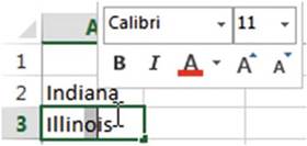
Figure 4-56. Smaller mini-toolbar
132
CHAPTER 4 ■ FORMATTING AND ALIGNING
DATA
The larger
mini-toolbar shown in Figure 4-57 includes
buttons from the Font, Alignment, and Number groups along
with the Format
Painter from the Clipboard group.
This mini-toolbar can be accessed
by right- clicking
any cell even if the cell is empty.
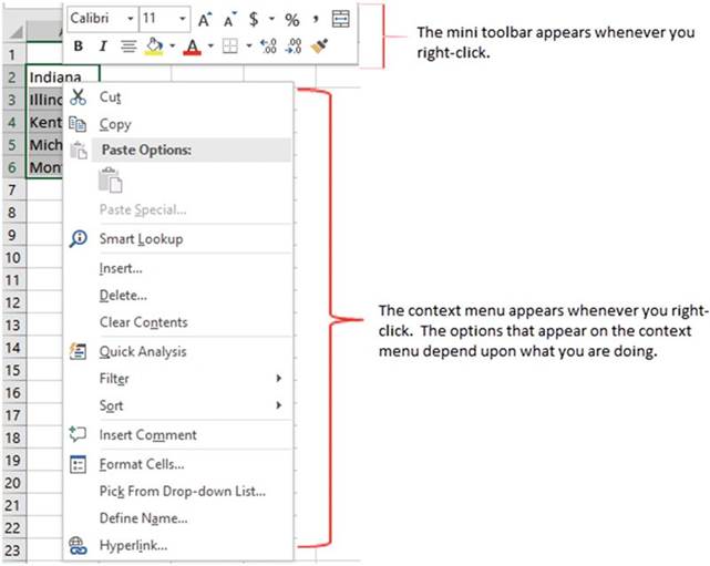
Figure4-57.Contextmenuandlargermini-toolbar
A context menu (also known as a shortcut menu) is also displayed when you right-click a cell or an object.
What items are displayed
in the context menu depends
upon the object you clicked
and what you are working
on at the time. You can make a selection
from either the mini-toolbar or the shortcut
menu. If you decide you don�t want to use either one just click another cell and they both will disappear.
Notice that the context menu has some options that have three
dots after them.
See Figure 4-58. The three dots are called
an ellipsis. The ellipsis signifies that another dialog
box will be opened when this option
is selected. For example, clicking
the Insert� option
on the context menu will bring up the Insert window. Some of the options on the context
menu have an arrow. Moving
your mouse pointer
over an arrow brings up a submenu
of additional options.
133
CHAPTER 4 ■ FORMATTING AND ALIGNING
DATA
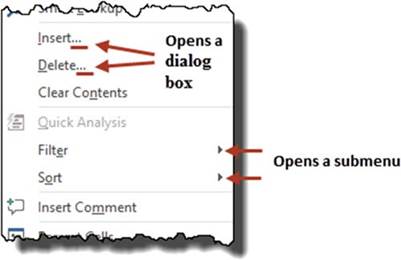
Figure 4-58. Context menu
Inserting, Deleting, Hiding, and Unhiding Rows and Columns
You can add new blank rows between
existing spreadsheet rows. You can also delete rows to remove data or
to remove blank rows.
You can hide a single
row or multiple rows of data from the view of users.
Rows that have been hidden can be unhidden. You don�t have to unhide
all the rows only the ones you choose.
Hiding and Unhiding
Columns and Rows
Columns and rows can be hidden and unhidden so that the users can concentrate on only the data that is
necessary and relevant to them.
Hiding Columns and Rows
There are many reasons for hiding columns
or rows in a spreadsheet.
�
There is too much data to display on a single
screen so you hide the data you really
don�t need to see.
�
You want to hide some of the data so it is
not printed.
�
The data is not relevant to the user.
�
You want to hide the formulas.
�
You don�t want the user to see some of the
data.
Hiding a column or row does not affect the data in that column or row, nor does it prevent it from being
referenced.
A single column or row of data can be hidden
as well as multiple columns
or rows. If you are hiding multiple
columns or rows they do not need to be adjacent.
How to
hide a single column or row
1.
Right-click the
column or row header.
2.
Select Hide from
the context menu.
134
CHAPTER 4 ■ FORMATTING AND ALIGNING
DATA
How to hide
adjacent columns or rows
1.
Drag across the
headers of the columns or rows you want to hide.
2.
Right-click the
selected headers.
3.
Select Hide from
the context menu.
How to
hide nonadjacent columns and rows
1.
Click a column
header.
2.
Hold down the
Ctrl key while you click other column heads.
3.
Right-click one of the selected column heads.
4.
Select Hide from
the context menu.
Use the same steps that you do for nonadjacent columns.
■
NoteYou can�t select columns
and rows in the same operation. You must first hide either columns or rows and then do the other.
Unhiding Columns and Rows
Columns and rows that you hide will remain hidden until you run the Unhidecommand.
Unhide All
Columns and Rows
You can unhide all columns and rows by first clicking
the Select All button located to the left of row head
A and then right-clicking any header and selecting Unhide
from the context
menu. If you wanted to unhide columns and rows from multiple
worksheets, you would
select those sheet
tabs before performing these steps.
Unhide Adjacent Columns or Rows
In the worksheet example shown in Figure 4-59 columns B and C are hidden.

Figure4-59.ColumnsBandCarehidden
Columns B and C can be
unhidden by dragging across Column heads A and D, right-clicking, and then
selecting Unhide.
Rows would be unhidden using the same steps, except of course you would use the Row heads rather than the
Column heads.
Unhide Nonadjacent Columns or Rows
In the worksheet example
shown in Figure
4-60 columns B and C are hidden, and so are columns F, G, and H.

Figure4-60.ColumnsBandC,F,G,andHarehidden
135
CHAPTER 4 ■ FORMATTING AND ALIGNING
DATA
Columns B and C and columns
F, G, and H can be unhidden
by dragging across Column heads A and D and then holding
down the Ctrl key while dragging across Column heads E and I, right-clicking, and then selecting Unhide.
Another way to accomplish this would be to unhide all five columns at once. You could drag across
Column heads A to I. Right-click one of the selected column heads and select Unhide.
Unhide Column A or Row 1
Unhiding
Column A or Row 1 is a unique situation. It is unique
because there is no column
head before Column A to drag across,
nor is there a row head before
row 1 to drag across.
Unhide Column A
1.
Type A1 in the Name Box and then press Enter.
2.
Click the Home
Tab on the Ribbon.
3.
In the Cells
group click the Format button.
4.
Select
Hide & Unhide from
the menu and then select Unhide Columns. See Figure 4-61.
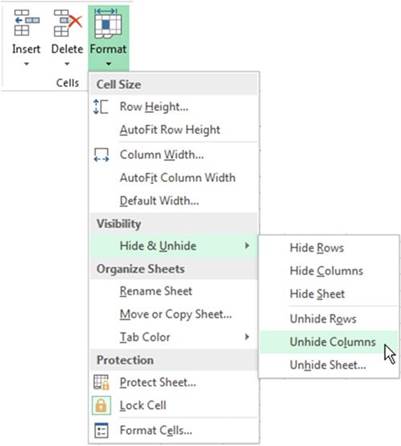
Figure 4-61. Hide & Unhide options
136
CHAPTER 4 ■ FORMATTING AND ALIGNING
DATA
Unhide Row
1
1.
Type A1 in the Name Box and then press the Enter key.
2.
Click the Home
Tab on the Ribbon.
3.
In the Cells
group, click the Format button.
4.
Select Hide & Unhide
from the menu and then select Unhide Rows.
This exercise takes you through hiding and
unhiding rows and columns as well as dealing with the unique issue of unhiding column
A and row 1.
1.
Create a new worksheet. Name it �Rows_Columns.�
2.
Type 1 in cell A1 and 2 in cell A2.
3.
Drag across cells A1 and A2 to select them.
4.
Drag the Autofill Handle down to row 12. Let go of the mouse button. See Figure 4-62.
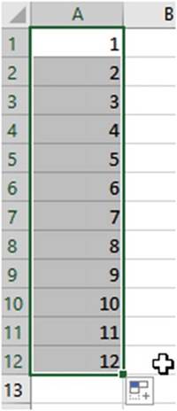
Figure4-62.CopiedpatternofcellA1andA2downthroughcellA12
137
CHAPTER 4 ■ FORMATTING AND ALIGNING
DATA
5.
Drag the Autofill Handle to the
right to column M. See Figure 4-63.
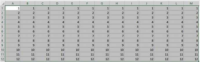
Figure4-63.CopiedcolumnAdatabyusingAutoFillHandle
Hide
Columns
1.
Drag across column heads B through D.
2.
Hold down your Ctrl key while you click column head G and
drag across column heads J and K.
3.
Right-click one of the selected column heads and then select Hide.
Hide Rows
1.
Drag across row heads 2 and 3.
2.
Hold down your Ctrl key while you drag across row heads 6
and 7 and click row head 10.
3.
Right-click one of the selected row heads and then select Hide.
Unhide
Columns
1.
Drag across column heads A and E. Right-click the selected area and then select Unhide.
2.
Drag across column
heads F through
L. Right-click the selected
area and then select Unhide.
Unhide
Rows
1.
Drag across row heads 1 through 12.
2.
Right-click the selected area and select Unhide.
Hide
Column A
1.
Right-click column head A.
2.
Select Hide.
138
CHAPTER 4 ■ FORMATTING AND ALIGNING
DATA
Unhide
Column A
1.
Type A1 in the name box and
then press Enter.
2.
Click the Home Tab on the Ribbon. In the
Cells group click
the Format button.
3.
Select Hide & Unhide from the menu and then select Unhide Columns.
Hide Row 1
1.
Right-click row head 1.
2.
Select Hide.
Unhide Row
1
1.
Enter A1 in the name box and
then press Enter.
2.
Click the Home Tab on the Ribbon. In the
Cells group click
the Format button.
3.
Select Hide & Unhide from the menu and then select Unhide Rows.
Inserting
Columns and Rows
After you have entered data into your workbook you may discover
that you need to add a column of data between your other columns
or maybe you want to add a blank column to make your worksheet
easier to read. The same holds true for rows, you may discover
that you forgot to add rows of data or you merely want
to add additional blank rows to improve
the appearance of your worksheet.
You can add a new
column(s) or row(s) anywhere in your worksheet.
How to
Insert Columns
1.
Select the column head where you want the column inserted.
2.
Right-click the worksheet and select Insert.
The column you selected will be shifted
to the right and the column that you created
will take its place. The new column will have the same width as the column to the left of it.
You can insert multiple
columns by selecting
the columns where you want the new ones inserted.
If you selected four columns,
then four new columns will be inserted
when you right-click the worksheet and select Insert.
How to Insert Rows
1.
Select the row
head where you want the row inserted.
2.
Right-click the worksheet and select Insert.
The row you selected will be shifted down and the row that you created will take its place. The new row will
have the
same height as the row above it.
You can insert multiple
rows by selecting the rows where you want the new ones inserted. If you
selected four rows, then four new rows will be inserted when you right-click the worksheet and select
Insert.
Deleting
Columns and Rows
You can just as easily remove
a column or row as you can add them.
Some of the reasons for removing a column would
be that
139
CHAPTER 4 ■ FORMATTING AND ALIGNING
DATA
�
You have entered the wrong data into a
column.
�
You have determined that you no longer need the data in a column.
�
You want to remove empty columns to improve the appearance or use of your spreadsheet.
If you entered invalid
data in a column it might be easier just to clear the data from the column rather than deleting
the entire column.
This could be done by selecting all the cells containing the invalid data, then selecting
Home tab | Editing Group | clear button
 , and then selecting one of the clear options.
How to
Delete Columns
You can delete one column or multiple
columns at the same time.
1.
Select the
column heads of the columns you want to delete.
2.
Right-click the worksheet and select Delete.
The columns to the right
of the deleted columns will be shifted
left to replace
those columns that you deleted
(to replace the vacated space).
How to
Delete Rows
You can delete one row or multiple
rows at the same time.
1.
Select the row
heads of the rows you want to delete.
2.
Right-click
the worksheet and select Delete. The rows below the deleted columns will be shifted up to replace those rows
that you deleted.
Inserting and Deleting
Cells
You can insert blank cells above or to the left of an active cell. You can bring up the Insert dialog box
(Figure 4-64) to perform this operation by right-clicking any cell and then selecting Insert from the
context menu.
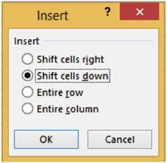
Figure 4-64. Insert window
When you insert blank
cells, you can choose to move the other cells
in the same column down (Shift
cells down) or to move the other
cells in the same row to the right (Shift
cells right) to accommodate the new
cells. Notice that the Insert
Dialog Box also has options
for inserting entire
rows and columns.
140
CHAPTER 4 ■ FORMATTING AND ALIGNING
DATA
You can remove cells by selecting
the cells you want to remove, then right-clicking and selecting Delete from the context menu. This brings up
the Delete Dialog Box (Figure
4-65) which provides
options for deleting cells, entire rows, or entire columns.
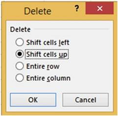
Figure 4-65. Delete window
You can choose to have the deleted cells replaced with cells from the right (Shift cells left) or you can
choose to have the deleted cells replaced with those from below (Shift cells up).
This exercise takes
you through inserting and deleting cells
and then deciding
how the other
cells need to be shifted
over.
1.
Create a new worksheet. Name the worksheet �Stocks.�
2.
Type Stocks Purchased 06-15-2016 in cell A1. Select cells
A1 to D1. Right-click the selected cells.
The larger mini-toolbar should appear above
your selected text. Click the Merge &
Center button
 .
.
3.
Type Stock in cell A2.
4.
Type Closing in cell B2. Press Alt + Enter. Pressing
Alt + Enter creates an additional line in the cell and turns on text wrapping.
Type Price.
5.
Select cells C2 and D2. Right-click in the selected
area. Select Format
Cells. Select Wrap text from the Alignment tab. Click the OK button.
6.
Type the data from Figure 4-66 in
cells C2 and D2. You may need to
widen your column to see all of the word Purchased. Then type the rest of the data in Figure 4-66.
141
CHAPTER 4 ■ FORMATTING AND ALIGNING
DATA
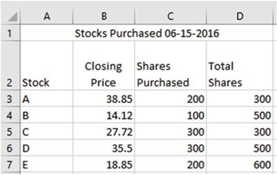
Figure4-66.Typethedatafromthisworksheet
7.
Right-click column head A and then select Insert from the context menu.
8.
Right-click row head 1 and then select Insert from the context menu.
9.
Right-click cell B5 and then select Insert. Select Shift cells down. Click the OK button.
10.
Right-click cell B5 and then select Delete. Select Shift cells up. Click
the OK button.
11.
You can select
multiple cells before
you select to shift the cells down or to the right.
The number of cells shifted
over will be the same number of cells you selected.
a.
Select cells B5:D5. Right-click
cell in the selected area and then select Insert.
b.
Select Shift cells right. Click the OK button.
12.
Right-click the three cells that are still selected and
then select Delete. Select Shift
cells left. Click the OK button.
13.
Right-click cell B4 and then select Insert.
Select Entire row. Click the OK button.
A row is inserted above
the selected cell.
14.
Right-click cell C4 and then select Insert.
Select Entire column.
Click the OK button. A column is inserted to the left of the selected cell.
15.
Right-click cell C4 and then select Delete. Select Entire column. Click
the OK button.
16.
Click row head 6. Hold
down your Ctrl key and click row heads 7, 8, and 9. Right-click any of the selected
row heads and then select Insert.
You should
now have a blank row between each of your rows.
■
NoteWhen making
selections your selected rows, columns, or cells do not have to be adjacent.
142
CHAPTER 4 ■ FORMATTING AND ALIGNING
DATA
You have learned
how to insert and delete rows and columns as well as how to hide and unhide them. You should only let users
who actually need to view the data access to it; you should hide anything that they don�t require. You also
learned
to insert and delete individual cells. You will often discover
that you forgot to make an entry. Excel makes it easy to correct
this oversight by letting you insert a new cell where it is needed and then moving the data below it down
one row or moving the data to the right of it over one column.
Summary
Formatting a worksheet
can make it more visually
appealing and easier to understand. It can also be used to change how numeric
and date data are displayed. Formatting can be used to create word wrapping, rotating
text, and shrinking
text. Formatting is also used to align data. You can use Excel�s Format Painter to copy all the formatting
applied to a cell to other cells. You�ve practiced
using color effectively and learned how to create a uniform
graphic style for worksheets. This is an important aspect of developing presentations that are professional
in appearance and providing a signature look for your projects. Excel makes formatting easier by providing
quick access to the tools you need most often by placing
them on two mini- toolbars.
You have seen how to hide and unhide rows and columns
and how to insert and delete cells, rows, and columns. You have also seen how to apply borders and how to
draw them.
In Chapter 5, you�ll continue to refine how the workbook
is set up by using headers and footers, setting the page breaks, dividing
worksheets into multiple
panes, and learning
more functions. You�ll also be learning about custom views and how to print select portions
of the worksheet for specific
data reporting purposes.
143
CHAPTER
5
Different
Ways of Viewing and Printing Your Workbook
Excel allows you to enter a
tremendous variety and amount of data into one worksheet and then extract only the data you need to share
with
clients or employees. Sometimes you don�t need to print the entire workbook or the entire worksheet. In
this chapter you�ll be learning how to view and print only the data relevant to your task. You may be
dealing with a geographic area or a particular salesperson and you only want to show what is relevant to
each
person. Print layout view lets you see how worksheets will look when printed, which is very important
because screenshots can be quite different from the final printed product.
After
reading and working
through this chapter
you should be able to
�
Insert, remove, reset,
and change the location of page breaks
�
Repeat row and column headers
on all pages
�
Use preset headers
�
Create your own headers and footers
�
Create a print
area, add to it, and remove it
�
Print a portion of a worksheet
�
Use Paste Special
to assemble a printable worksheet
�
Create your own custom views
�
Use the Synchronous Scrolling feature
�
Divide a worksheet into multiple panes
�
Freeze rows and columns
Views
So far we have been looking
at the worksheets in the Normal view, but this isn�t the only view available. In addition to the
Normal
view, there is a Page Break Preview
and a Layout view. The
different views can be accessed
from the View tab on the Ribbon.
Page Break
Preview is used for adjusting page breaks. This view lets you insert,
change, remove, and reset page breaks. Page Layout view provides a quick way to add, edit, and delete
headers
and footers. It also lets you visualize how your workbook
will look when printed. You can also create your own custom views.
The Workbook
Views are located
on the Ribbon�s View Tab. See Figure
5-1.
145
CHAPTER 5 ■ DIFFERENT WAYS OF VIEWING AND PRINTING YOUR
WORKBOOK
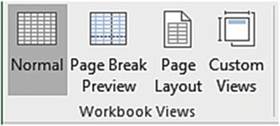
Figure 5-1. Workbook View buttons
The Normal view, Page Break Preview,
and Page Layout view buttons
also appear on the right side of Excel�s
task bar. These three buttons
 �perform the same functions as those in the Workbook View group. If you do not see them on your
task bar, right-click the task bar and select View Shortcuts.
�perform the same functions as those in the Workbook View group. If you do not see them on your
task bar, right-click the task bar and select View Shortcuts.
■
Note� Normal view and Page Break Preview do not display
headers and footers
but Page Layout view does.
There is also a Print
Preview which you will use in this chapter. The Print Preview
is not a part of Workbook views.
Print Preview is only used for seeing
exactly how your worksheet will be printed.
Page Break Preview
There are two types of page
breaks: those that are created automatically by Excel and those you create manually. Automatic page breaks
adjust
whenever you do such things as change the row height or column width, delete or add columns or rows,
change page size, change page orientation, change margins, and so on.
In Normal view page breaks appear as dashed lines. In Normal view you can insert, remove, and reset
page breaks. You can�t, however, drag page breaks to a new location like you can in Page Break Preview.
Page break lines are also much easier to see in Page Break Preview. The way you insert, remove, and reset
page breaks is done the same way in both Normal and Page Break Preview. Therefore, we will only look at
performing these steps in the Page Break Preview mode.
Printing a worksheet that contains a lot of columns can be a challenge. Excel
may not be breaking up your report
(printed worksheet) the way you want it to. You can change
from Portrait to
Landscape
orientation so that you have more width to your paper but you still may end up with some columns printing
on a separate page. Page Break Preview is used for adjusting page breaks. This view lets you insert,
change,
remove, and reset page breaks.
Page Break
Preview shows a minimized view of your data. The data is separated by
horizontal and
vertical blue
dashed lines that represent page breaks. You can change the location of a page
break by dragging a blue line to
where you want the break to occur. If you change the location of a page break,
the line changes from a dashed line
to a solid line. If you insert a new page break, it will also display as a
solid line.
This makes it easy to identify changes that you have made from the page breaks that Excel originally created.
In this exercise you will practice creating
vertical and horizontal page breaks. You
will also practice moving and
removing them.
146
CHAPTER 5 ■ DIFFERENT WAYS OF VIEWING AND PRINTING YOUR
WORKBOOK
■
Note� You can download the sample files included with this book from the Source
Code/Download area of the Apress web site (www.apress.com/9781484221600).
1.
Open the workbook Chapter 5. Click the Months worksheet.
2.
Click the File tab.
3.
Select Options in the left pane.
4.
Select Advanced in the left pane.
5.
Look for the Display options for this worksheet group. If the Show page breaks isn�t checked, then
check it.
6.
Click the OK button. This only affects
Normal view. You can�t turn off the Page Break lines in Page Break
Preview.
Now that Show Page Break is selected you should see page breaks that are represented by dashed lines. There
is a vertical page break between columns E and F and another vertical page break between columns J and K
(Figure 5-2). There is a horizontal page break between rows 47 and 48 (Figure 5-3).
Figure 5-2. Vertical page break line
Figure 5-3. Horizontal page break line
7.
Click the View tab on the Ribbon. In the Workbook View group click the
Page Break Preview button. The rest of the exercise pertains only to Page Break
Preview. Look at
the Zoom tool at the bottom right of your window. The zoom is automatically set lower
than 100% to make it easier to see your page breaks.
147
CHAPTER 5 ■ DIFFERENT WAYS OF VIEWING AND PRINTING YOUR
WORKBOOK
The worksheet displays
with two vertical
dashed lines and one horizontal dashed line separating the worksheet into six pages.
See Figure 5-4.
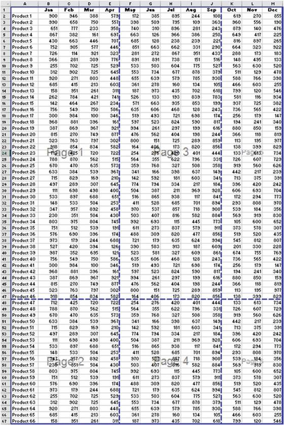
Figure 5-4. Page Break Preview
148
CHAPTER 5 ■ DIFFERENT WAYS OF VIEWING AND PRINTING YOUR
WORKBOOK
View the Report in Print Preview
1.
Click the File tab. Select
Print in the left pane. The Print
Preview pane on the right
shows how the worksheet would look when printed. You can click
the Forward and Back
buttons
 �at the bottom of the preview
area to view the different pages.
�at the bottom of the preview
area to view the different pages.
2.
Click the Return button
 �to leave Print
Preview.
�to leave Print
Preview.
Insert a
Page Break in Page Break Preview
1.
Click column head H so that the column is selected. When you insert
a vertical Page Break the break will occur to the left of the selected column.
2.
On the Ribbon
click the Page Layout tab. In the Page Setup group,
click the Breaks
button A
Remove a
Page Break in Page Break Preview
1.
Right-click column head H. Select
Remove Page Break.
2.
You can also remove a page break line by dragging it off the worksheet. Drag the vertical
page break between
columns J and K off the worksheet.
Reset Page
Breaks in Page Break Preview
1.
Right-click the
worksheet then select Reset All Page
Breaks. This puts the page breaks back to the way Excel originally
set them
Change the
Location of the Page Breaks in Page Break Preview
1.
Drag the horizontal page break line so that it falls between rows 36 and 37. This line turns into
a solid line. This makes it easy to identify
page separators that Excel set (dashed lines) and those that you set (solid lines).
2.
Drag the dashed break line that is between columns
E and F so that it is between columns
G and H. The line turns into a solid line.
View the
Spreadsheet in Print Preview
1.
Right-click the worksheet then select Page Setup. On the Page Setup dialog
box, click the Print Preview
button.
2.
The right side of the window is the Print Preview area. This shows exactly what your print out
would look like. At the bottom of the window
you will see a page selector.
 �Click the right arrow
to go to the next page. Notice
that on page two there
are no column headers. Click
the right arrow
of the page selector to go to page 3. Notice there
are no row headers. Go to page 4. This page has neither row nor column
headers. It would
be very difficult for anyone to read this report unless you taped
the pages together. See Figure 5-5.
�Click the right arrow
to go to the next page. Notice
that on page two there
are no column headers. Click
the right arrow
of the page selector to go to page 3. Notice there
are no row headers. Go to page 4. This page has neither row nor column
headers. It would
be very difficult for anyone to read this report unless you taped
the pages together. See Figure 5-5.
149
CHAPTER 5 ■ DIFFERENT WAYS OF VIEWING AND PRINTING YOUR
WORKBOOK
Figure5-5.Page4ofreporthasnoroworcolumnheadings
■
NoteWhen you viewed the spreadsheet in Page Break Preview it appeared with a grid but in
Print Preview
there is no grid. It would print without any grid lines.
3.
Click the Return button
�and then click the
Ribbon�s Home tab.
Repeat
the Row and Column Headers on All of the Pages
1.
Right-click the worksheet
and then select
Page Setup. On the Page Setup dialog
box, click the Sheet tab.
2.
If we want the row headings to appear on every printed
page we need to identify
the headings row in the Rows to repeat at top textbox. Click inside the textbox. You can type
$1:$1 in the textbox or you can click cell A1 and it will put the address in the textbox
for you. This address tells Excel to use the headings in row 1 as the column headings
for all of the printed
pages.
3.
Tab to the Columns
to repeat at left textbox. You
can type $A:$A in the textbox or you
can click cell A1 and it will put the
address in the textbox for you. This
address tells Excel to use the row headings in column A as the row headings for all printed pages.
4.
Select the check box for Gridlines. This will print all of the data within grid lines. See Figure
5-6.
150
CHAPTER 5 ■ DIFFERENT WAYS OF VIEWING AND PRINTING YOUR
WORKBOOK
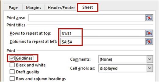
Figure5-6.SelectGridlinestoprintthedatawithingridlines
5.
Click the Print Preview button. The
page now displays with gridlines.
6.
Click the Zoom to
Page button located at the bottom right of the Print Preview area. See
Figure 5-7.

Figure 5-7. Click the Zoom to Page button
7.
Click the left arrow of the page selector until you are at page 1 of 4
 �. Page 1 shows the data for months January
through June. Click
the right arrow of the page selector
to go to page 2. Page 2 shows the remaining records
for months January
through June. Page 2 now has column headers.
�. Page 1 shows the data for months January
through June. Click
the right arrow of the page selector
to go to page 2. Page 2 shows the remaining records
for months January
through June. Page 2 now has column headers.
8.
Go through the other pages; they all have column and row headers.
9.
Click the Return button
�.
You have learned how to insert, remove, and rearrange page breaks so that you can control where page breaks
occur. You also learned how to make the row and column heads appear on each page of a report.
Next,
you will see how to add headers
and footers to your worksheets in the Page Layout View.
Page
Layout View
Page Layout view provides a
quick way to add, edit, and delete headers and footers. It shows what your printout will look like relative
to a
horizontal and vertical ruler along with the breaks between pages. You can easily change margins and then
instantly see the results. Page Layout view works similar to Normal view; you can still add and edit data
and apply
formatting.
151
CHAPTER 5 ■ DIFFERENT WAYS OF VIEWING AND PRINTING YOUR
WORKBOOK
Page Layout
view displays a horizontal ruler and vertical ruler that moves to another page
when you move to another page. You
can adjust your borders by dragging the ruler to the location you want. As you
are dragging your mouse
pointer, a line moves at the same time showing you where the margin is. If you
want your margin at a certain
inch this is not the place to do it because it doesn�t display the change in
inches as you are dragging.
The Page Layout view displays three header sections, and three footer sections. If you click one of the
header or footer sections, a new contextual tab will be added to the Ribbon named Header & Footer
Tools.See Figure 5-8. A header prints at the top of each page. A footer prints at the bottom of each
page.
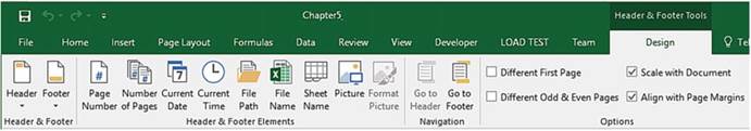
Figure5-8.Contextualtabforheadersandfooters
In this exercise
you will use the Page Layout View to add and change
headers and footers
and to remove whitespace between
pages.
1.
Use workbook Chapter 5. Click the Months worksheet.
2.
Click the Page Layout view button
 �on the Workbook�s status bar.
You should
see on the status bar that we are looking at page 1 of 4.
3.
Change the Zoom tool so that you can see all pages at the same time.
4.
Press Ctrl + Home to go to cell A1.
Change
the Header and Footers
1.
Change the Zoom tool so that you can see the text Add Header above
the worksheet. Move your mouse pointer to the Add header
text. The section
should be selected.
See Figure 5-9.

Figure5-9.Addaheadertotheworkbook
2.
Move your mouse pointer to the left of that section and the
left section will be selected. Click inside the left section. Whenever a Header or Footer section is
active the Ribbon will have a Design tab
appearing under the heading Header and
Footer Tools.
152
CHAPTER 5 ■ DIFFERENT WAYS OF VIEWING AND PRINTING YOUR
WORKBOOK
3.
Click the Design
tab. In the Header & Footer group, click the Header button.
Excel displays a list of preset headers.
See Figure 5-10.
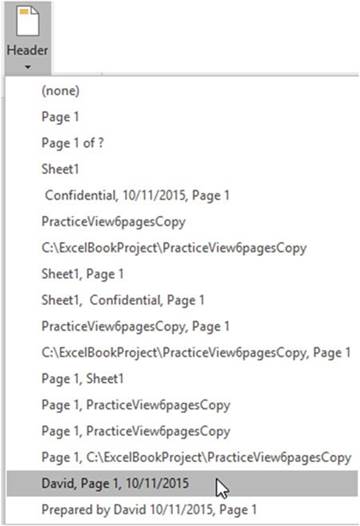
Figure 5-10.Select
a header from one of these preset headers
The data
that will print in each section of the header is separated by commas:
�
The preset headers that contain no commas will display in
the middle header section.
�
For those that contain one comma, the text to the left of the comma will appear in the middle
Header section. The text to the
right of the comma will appear in the right
section.
�
For those that contain two commas, the text to the left of the first comma will appear in the
leftmost Header section. The text to
the right of the first comma will
appear in the middle section. The
text to the right of the second comma will appear in the right-most section.
4.
Click the preset header that consists of the username, the page number, and the current date.
153
CHAPTER 5 ■ DIFFERENT WAYS OF VIEWING AND PRINTING YOUR
WORKBOOK
5.
Click inside the first header
section and change
the name to your full name. Use the worksheet�s vertical and horizontal scroll bars to see that the header
appears at the top of each page.
6.
Scroll to the bottom of page 1. You
should see the text Add footer.
7.
Click the words Add Footer so
that you can see the three footer sections.
8.
Click the Design
Tab. In the Header & Footer group,
click the Footer button.
Excel displays a list of preset footers. Just like with the headers the commas are
used to identify which section the text will go in.
9.
Click the preset footer Page 1 of ?. The preset
footer didn�t contain a comma; therefore it displays in the middle section.
10.
Click inside the middle section.
The code Page &[Page] of &[Pages] used
to create the footer is displayed. We would prefer the text to appear in the right section.
Press Ctrl + X to cut the text. Click inside the right section. Press Ctrl + V to paste it. Click
inside the middle section. You should now see the text in the right section.
11.
Click the Ribbon�s
Design tab, in the Navigation group, and then click the Go to Header
button.
Print
the Worksheet
1.
Click the Ribbon�s File tab. Click
Print in the left pane.
2.
You should see the worksheet
with three headers.
Scroll down to the bottom
of the page if you need to, to see the footer
Page 1 of 4. Go through
the other pages. The headers
and footers are the same on each page.
3.
Click the Print button if you want to print the report.
4.
Click the Return button
.
Change
the Scale and Alignment of your Headers and Footers
1.
Click any one of the three Header sections at the top
of the page. Click the Design tab.
The Options
group (Figure 5-11) contains options for your headers and footers:
�
One option is for making
one set of headers and footers for the first
printed page while
all of the other pages
will have a different set of headers
and footers.
�
Another option is to have one set of headers
and footers for the odd pages and another set for the even pages.
�
The Scale with Document option when selected
scales the size of the headers and footers so that they are proportionate to any changes
you made to the print scale to fit in more or less information on your printed
page.
�
The Align with Page Margins
when selected places
the headers and footers within the page margins that you set up.
154
CHAPTER 5 ■ DIFFERENT WAYS OF VIEWING AND PRINTING YOUR
WORKBOOK
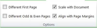
Figure 5-11.Options for how you want your headers
and footers to appear
2.
Remove the check
mark for the Align with Page Margins option; as you do so, notice
how your header
spreads out.
3.
Remove the check mark for Scale with Document. Notice
how your header text increases in
size.
4.
Turn the Scale with Document and
Align with Margins back on.
5.
Select Different First Page if
it isn�t already selected.
6.
On the Ribbon�s
Design tab in the Header
& Footer group and then click the Header button.
Select Months, Confidential, Page 1.
7.
Click inside the Page Header area to see the results.
8.
Scroll through the pages; you will see that only the first page header has
changed.
9.
Click the Page Header area for page 1.
10.
On the Ribbon�s
Design tab in the Options
group, remove the check from Different First Page.
11.
Click Different Odd & Even
Pages.
12.
Click the Left Header section
on Page 1 and change
the text to Accounting Department.
13.
Scroll down to page 2. Click
inside the Page Header Section.
14.
Click the Ribbon�s
Design tab. In the Header
& Footer group,
click the Header
button. Select Page 1 of ?.
15.
Click inside the Page Header area to see the results.
16.
Scroll through the pages. You should see that the headers are different for odd and even pages.
Remove
Whitespace Between Pages
There is a lot of whitespace between
each of our pages. Removing
the whitespace would
make the worksheet easier to read.
1.
Move your mouse pointer to the vertical blank space between
pages 1 and 3 and click. See Figure 5-12.
155
CHAPTER 5 ■ DIFFERENT WAYS OF VIEWING AND PRINTING YOUR
WORKBOOK
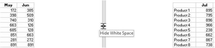
Figure5-12.Removewhitespacebetweenpages
2.
Scroll down. You should see that all of the whitespace between
the pages has been removed.
■
Note� The worksheet is easier to read now, but you can�t see the headers
or footers. Clicking
between the pages
will put the whitespace back.
You can again
view the headers
and footers.
Turn the
Show Options Off and On
1.
Click the View tab. In the Show group there are check
boxes for Ruler,
Formula
Bar, Gridlines,
and
Headings.
See
Figure 5-13.
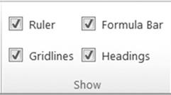
Figure5-13.TheRibbon�sShowgroupontheViewtab
2.
These
options only affect how the worksheet is displayed. They have no effect on how the worksheet
is printed. The ruler option is only available in Page Layout view. The Headings are the row numbers
and column head letters. Remove the check mark for each one of these options. As
you do so,
notice its effect. Then turn them all back on.
3.
Switch to Normal view by clicking the Normal View button
 �on the status bar.
You�ve used the Page Break Preview and Page Layout views. Now, you�ll return to the Normal view to see
different ways of selecting what you to want to print.
156
Printing
CHAPTER 5 ■ DIFFERENT WAYS OF VIEWING AND PRINTING YOUR
WORKBOOK
Spreadsheets
can be huge. Aligning the pages and getting the margins just the way you want
on a large spreadsheet can be
difficult. But chances are you don�t want to print all of the information from
a large spreadsheet. If you only
want to print a portion of a worksheet, you can do this in several ways.
�
Hide the rows or columns
you do not want to print.
�
If the cells that you want to print are not adjacent, you can select the cells from one area that
you want to print then hold down your Ctrl key and select other areas to print.
�
Copy the different ranges you want to print to another worksheet in the order that you want to see
it printed. You can use paste links so that the data is updated
dynamically. Then print the worksheet that contains only the data you want to print
in the order that you want to print it.
�
Set up print areas. Print areas can be expanded as needed or can be cleared. Only the print areas
will be printed unless you select the option to Ignore Print Area.
The following
sections will guide you through
using Print Areas and assembling a printed report
in the order you want.
Creating a Print Area
You can elect to print only the portions of the spreadsheet you need by selecting one or more ranges that
you want to print and then making those ranges a Print Area. Set up a Print Area if you will be
frequently
printing only those areas of the worksheet.
A Print Area can be set up by selecting the cells you want to print and then clicking the Print Area button
located in the Page Setup group on the Page Layout tab. See Figure 5-14. Selecting the Set Print Area
creates the print area. The Add to Print Area option only appears if you have already set up a
Print area.
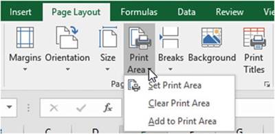
Figure 5-14. Print Area button
Excel saves the selected cells as a named range automatically naming it Print Area. You can only have one
Print Area but the Print Area can contain multiple ranges.
157
CHAPTER 5 ■ DIFFERENT WAYS OF VIEWING AND PRINTING YOUR
WORKBOOK
Adding Additional Cells to the Print Area
Additional Cells can be added to the Print
Area after you have created
it by selecting those cells and then clicking the Print Area button and selecting Add to Print Area.
■
Note� There is one irritating problem
when using multiple
ranges for Print Areas and that is Excel places a page break between
the ranges. This means that each addition
to the Print Area will appear on a separate
page.
Removing the Print Area
The Print Area can be removed by simply clicking
the Print Area button and then selecting
Clear Print Area.
You would only
use a Print Area if you were going to use it multiple times; otherwise you
could select the areas you want to print
and then click the Ribbon�s File tab, select Print from the left pane, click
the down arrow for Print Active
Sheets, and then select Print Selection. See Figure 5-15.
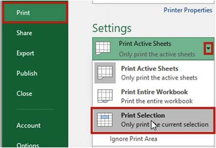
Figure5-15.Printonlytheselectedareaoftheworksheet
The worksheet for this example contains data
for a large corporation that is tracking sales for thirty-nine products sold in
17 of its stores.
1.
Open the workbook Chapter 5, which you have been using for this
chapter, if it isn�t currently open. Click the Stores worksheet.
2.
Drag across column heads D through G. Right-click one of the selected column
heads. Select Hide.
158
CHAPTER 5 ■ DIFFERENT WAYS OF VIEWING AND PRINTING YOUR
WORKBOOK
3.
Drag across column heads L through R. Right-click one of the selected column
heads. Select Hide.
4.
Click the Ribbon�s File tab. Select
Print from the left pane.
5.
Notice that the hidden columns do not appear in the print preview.
6.
Click the Return button
.
7.
Add the data in Figure 5-16 to the worksheet as shown starting in cell U3.
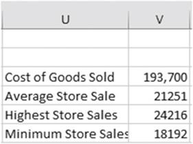
Figure5-16.Addthisdatatotheworksheet
8.
Select cells A1 through H9 (A1:H9).
9.
On the Ribbon�s
Page Layout
tab in
the Page
Setup group
click the
Print Area button then select Set
Print Area.
The name Print Area should
appear in the Name box.
10.
Select cells U3 through V6 (U3:V6). You should see a thin line around
the cells A1:H9 indicating that you selected
those cells for the print area.
11.
In the Page Setup group click
the Print Area button and select Add to Print Area.
12.
On the Ribbon click the File tab. Select
Print from the left pane.
13.
The print preview
area should show that you are looking
at page 1 of 2. The cells you selected
when you clicked
on Add to Print Area are on the second
page. Every time you use Add to Print Area to
add another selection
it will print on a different page. If you want each section on a separate
page, this works great; however,
if you do not, you can use Paste Special
which is discussed in the next section.
■
Note� If you change Settings to Print Entire Workbook
the Print Area will be ignored and the entire
workbook will be printed. If you select Ignore Print Area the Print Area will not be recognized by
any of the Print options. See Figure 5-17.
159
CHAPTER 5 ■ DIFFERENT WAYS OF VIEWING AND PRINTING YOUR
WORKBOOK
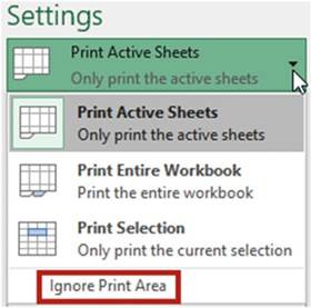
Figure 5-17.Select Ignore Print Area to prevent any
print options from using the Print Area
14.
Click the Return button
 .
.
15.
On the Ribbon�s
Page Layout tab in the Page Setup
group click the Print Area button then select Clear Print
Area.
16.
Unhide the hidden columns.
You�ve learned how to print only the cell ranges that you want to print. Next, you will see how using
Paste Special gives you more control over printing and helps overcome the problem of Excel placing page
breaks between ranges.
Using Paste Special for Printing
If you want more control of
where the different sections of your report will print, you can copy the
sections you want to see in a report
and then use Paste Special to place them on a separate worksheet in the
location that you want them printed.
Another benefit of this is that you can copy the data from different
worksheets.
In this exercise you will take different
portions of a worksheet and assemble them on another worksheet which can be printed as a single page.
1.
Use the Chapter 5 workbook. Create a new worksheet. Name the worksheet �Pasted.�
2.
Click the Stores
worksheet. Select the cell range A1:E9.
Press Ctrl + C to copy the data.
3.
Click the worksheet you named Pasted. Click
inside cell A1.
4.
On the Ribbon�s
Home tab in the Clipboard
group, click the down arrow of the Paste button.
Select Paste Special which
is the last option.
160
CHAPTER 5 ■ DIFFERENT WAYS OF VIEWING AND PRINTING YOUR
WORKBOOK
5.
The Paste Special
dialog box displays. Click Paste Link. See Figure 5-18. This creates a link between
the data on the Stores
worksheet and the data on the Pasted
worksheet.
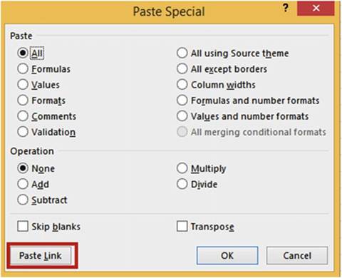
Figure 5-18.Paste
Link creates a link between
the copied and pasted data
6.
Click the Stores worksheet. Select the range U3:V6. Press Ctrl + C to copy the data.
7.
Click the worksheet
you named Pasted.
Click in cell G2. On the Ribbon�s
Home tab in the Clipboard group, click the down arrow of the Paste button.
Select Paste Special.
8.
The Paste Special
window displays. Click Paste Link. Widen column G to see all the data.
9.
Click the Stores worksheet. Select the range A17:D21. Press Ctrl + C to copy the data.
10.
Click the worksheet
you named Pasted.
Click inside cell A11. On the Ribbon�s
Home tab in the Clipboard group, click the down arrow of the Paste button.
Select Paste Special.
11.
The Paste Special window displays. Click
Paste Link.
12.
On the Ribbon,
click the File tab. Select
Print from the left pane. The print preview shows that you have managed
to get the data you want in the location
you want and still keep it on the same page.
13.
Click the Return button
.
161
CHAPTER 5 ■ DIFFERENT WAYS OF VIEWING AND PRINTING YOUR
WORKBOOK
14.
Click the Stores worksheet. Change
the value in cell B2 from 900 to 820.
15.
Click the Pasted worksheet. Because
you created a link cell B2 was updated with the
value you entered
on the Stores worksheet.
You�ve learned how using
Paste Special gives
you more control
over printing than using Print
Areas.
Paste Special allows you to take data from multiple areas and arrange it in the order that you want to print
it.
Next, you will see how to view multiple copies of your worksheet at the same time.
Dividing the Excel Window into Panes
Large worksheets can be difficult to analyze. You can�t see your column heads and your column totals
at the same time; therefore, whenever you�re looking at a total you have to scroll back to the top of the
worksheet to view its column heading in order to know what the total represents. The same thing applies
to your row totals and row headings. Another potential problem is that you want to compare the values in
Column B with the values in
column V but you can�t see both of them at the same time, so you have to scroll horizontally back and forth
to do your
comparisons. These types of problems can be solved by dividing your Excel screen into separate panes. A
copy of your worksheet is automatically placed into each of the panes you create. This gives you the benefit
of being able to view different areas of the worksheet at the same time.
The screen
can be divided into two vertical panes,
two horizontal panes,
or a combination of the two which
would give you four panes.
Here is how to create two vertical panes:
1.
Click a column head.
2.
Click the Ribbon�s View tab. In the Window group, click the Split button. See figure 5-19. The
pane will split to the left of the selected column.
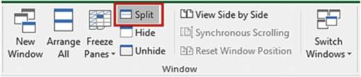
Figure5-19.SplitWindowbuttonishighlighted
Here is how to create two horizontal panes:
1.
Click a row head.
2.
Click the Ribbon�s View tab. In the window
group, click the Split button.
The pane will split above
the selected row.
Here is how to create four panes:
1.
Click a cell.
2.
Click the Ribbon�s View tab. In the window group, click the Split button. Split Bars appear above
and to the left of the selected cell. See Figure 5-20.
162
CHAPTER 5 ■ DIFFERENT WAYS OF VIEWING AND PRINTING YOUR
WORKBOOK
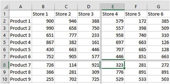
Figure 5-20.Window
split into 4 panes. Split is above and to the left of selected
cell
The
size of the panes can be adjusted
by dragging the split bars to the location you want.
If no Splits
bars are currently displayed, then clicking the Split button will display a
horizontal and vertical bar at the center of the window (not the
worksheet). See Figure 5-21.
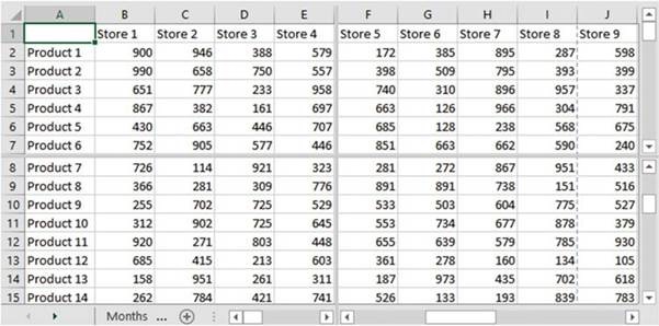
Figure5-21.Splitbarsappearatthecenterofthewindow
Placing a
horizontal split bar on a worksheet adds an additional vertical scroll bar.
Placing a vertical split
bar on a worksheet adds an additional horizontal scroll bar. Placing a
horizontal and vertical split bar on a worksheet adds an additional horizontal and vertical scroll bar. This
provides the capability to scroll through each pane individually. See Figure 5-22.
163
CHAPTER 5 ■ DIFFERENT WAYS OF VIEWING AND PRINTING YOUR
WORKBOOK
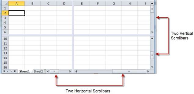
Figure 5-22.Horizontal and vertical scroll
bars for separate
scrolling of the four panes
A split bar can
be removed from the worksheet by double-clicking it. You can remove both split
bars at the same time by
double-clicking the area where the two split bars meet. The Split button on the
Ribbon works like a toggle switch.
Click it to add split bars. Click it again to remove the split bars.
Freezing Rows and Columns
Freezing rows and columns is another way of resolving the problem of not being able to view your row headings
and row totals at the same time or your column headings and column totals at the same time.
You
can select one of three
options when freezing
your worksheet.
�
Freeze Panes. You can freeze both the columns and rows that come before the current cell.
If the current cell is C4 this means that columns A and B are frozen and rows 1, 2, and 3 are frozen. The
rest of the columns and rows are scrollable.
�
Freeze Top Row. You can freeze the top row of your worksheet
so that it remains visible
while scrolling through
the rest of the worksheet.
�
Freeze First
Column. You can freeze the first column
so that it remains visible
while scrolling through the rest of the worksheet.
You can select one of the three options by clicking the View tab then clicking the Freeze Panes button
located in the Window group. See Figure 5-23.
164
CHAPTER 5 ■ DIFFERENT WAYS OF VIEWING AND PRINTING YOUR
WORKBOOK
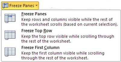
Figure 5-23. Freeze Pane options
Once you have frozen the worksheet using one of the three options, the first option will change from Freeze
Panes to Unfreeze Panes. Clicking Unfreeze Panes will return you to normal viewing.
Synchronizing Scrolling
You can use the New Window, View Side by Side, and Synchronous Scrolling options in the Window group to open
a second copy of your workbook and view the workbooks side by side with the same worksheets having
synchronized scrolling.
In this exercise
you will split a worksheet
into multiple worksheets. It appears as if there are multiple
copies of the worksheet, but they are just separate
views of the same worksheet
that you can scroll together. You will also practice freezing
rows and columns.
1.
Open workbook Chapter 5 if it isn�t opened already. Click the Stores worksheet.
2.
On the Ribbon�s
View tab in the Window
group, click New Window. A second window opens with the Stores
worksheet active. The name at the top of the workbook shows as Chapter
5:2. The original
workbook title bar shows Chapter
5:1.
3.
On Chapter 5:2, click the Ribbon�s view tab; in the Window group click View Side by Side.
4.
If you have other workbooks
open in addition to the Chapter 5 workbook a Compare Side by Side window appears
from which you can choose the workbook
you want to view side by side with it. You would select Chapter
5:1.
5.
Synchronous Scrolling is now highlighted under the View Side by Side button.
Use the vertical and horizontal scroll bars on one of the workbooks. Notice that as you drag the scroll bar
on one workbook
the other workbook
scrolls as well.
6.
Close one of the workbooks by clicking the X in the
upper-right corner of the workbook. The workbook title goes back to its
original name of Chapter 5.
165
CHAPTER 5 ■ DIFFERENT WAYS OF VIEWING AND PRINTING YOUR
WORKBOOK
Create
the Split Bars
1.
Click inside cell A3. On the Ribbon�s
View tab, in the Window
group, click the Split button.
A split bar appears above the currently
selected cell. You can drag the split bar to another location. Drag the horizontal split bar down so that it
is between rows 7 and 8. Notice
that you have two vertical
scroll bars. See Figure 5-24.
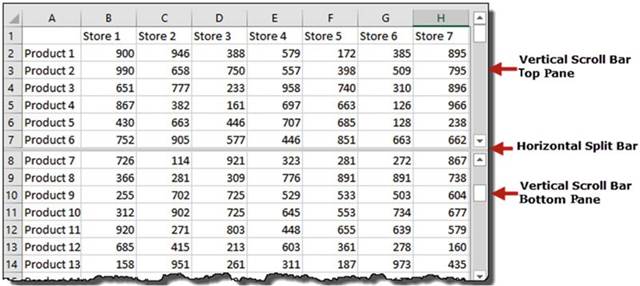
Figure 5-24.Window divided into two panes with two
separate scroll bars
2.
Use the scroll bar in the top pane to scroll through the data in the top
pane.
3.
Use the scroll
bar in the bottom pane to scroll
through the data in the bottom pane.
As you can see you have two complete copies
of your worksheet. Adjust your worksheets so that you can see cell B2 in both worksheets.
4.
Click inside cell B2 in the upper pane. When you select a cell in one pane it
also selects it in the other pane.
5.
Type 500 in the cell. Press
Enter. Cell B2 should now have a value of 500 in both worksheets.
6.
Double-click the split bar to remove it.
7.
Click cell G8. On the Ribbon�s View tab, in the Window group, click the Split button.
This creates intersecting split bars above and to the left of the cell. See Figure 5-25.
166
CHAPTER 5 ■ DIFFERENT WAYS OF VIEWING AND PRINTING YOUR
WORKBOOK
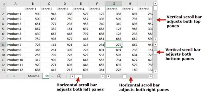
Figure 5-25.Window split into four panes with two
vertical and two horizontal scroll bars
Practice moving both horizontal and vertical scroll bars then adjust the four worksheets so that you can see
the same cell in all four panes. Click one of the cells.
Notice that it highlights the same cell in all four panes.
If you make a change to one of the cells, it affects the worksheet in all four panes.
8.
Move your mouse pointer where
both split bars meet. Your mouse pointer
should turn into a double
arrow. See Figure
5-26. Hold down your mouse
button and drag in any direction; both split bars will move with your mouse.
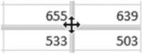
Figure 5-26.The
mouse pointer displays
as a double arrow when placed where
split bars connect
9.
Double-click where the two split bars meet to remove both of them.
167
CHAPTER 5 ■ DIFFERENT WAYS OF VIEWING AND PRINTING YOUR
WORKBOOK
Freeze
Panes
1.
In the Window
group click the Freeze Panes button. The three options
for freezing appear:
a.
Click the one for freezing
the top row. Scroll down through your data. The column headings
will remain in their fixed
location so that no matter
what row you are in you can always
see the column
headings.
b.
In the Window group click the Freeze Panes
button. The first option has changed to Unfreeze
Panes. Click this option to
remove freezing of the top row.
c.
Click the Freeze
Panes button. Click the one for freezing
the first column.
Scroll to the right to the end of your data. The row headings
will remain in their fixed
location so that no matter
what row you are in you can always see the row headings.
d.
Click the Freeze
Panes button. Click Unfreeze Panes.
2.
Click cell B2 and complete
these steps:
a.
Click the Freeze Panes button.
b.
Click Freeze Panes.
c.
Scroll through to the end of your data vertically and horizontally. Both your column
headings and row headings remain
stationary.
d.
Unfreeze the panes.
3.
Practice with a different active cell and then freeze the
panes. How does this affect the rows above and the columns to the
left of the active cell?
You�ve learned how to freeze row and column heads so they remain stationary as you scroll. You have also
learned to view multiple copies of your worksheet at the same time while keeping their scrolling
synchronized. Next, you will see how you can specify the different ways you want to view a worksheet and
then save those views as custom views.
Custom Views How to Create, Show, and Delete
If you or other users view
your workbook in different ways, such as with different headers or footers,
with different print areas or
different margins, with different columns or rows showing, or with the data
filtered, etc., you can save the
different views as custom views. Each custom view is assigned its own name.
When a custom view is opened it
opens with all of its stored settings.
Before you
create a custom view you need to set the workbook to appear exactly how you
want it to appear and how you want it
to print. When you are ready to save your current view, click the View tab. In
the Workbook Views group click
the Custom Views button. See Figure 5-27.
168
CHAPTER 5 ■ DIFFERENT WAYS OF VIEWING AND PRINTING YOUR
WORKBOOK
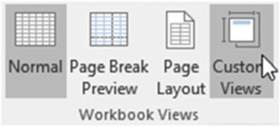
Figure 5-27. Custom Views button
Clicking the Custom Views button brings up the Custom Views dialog box shown in Figure 5-28 where you click
the Add button.
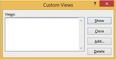
Figure5-28.CustomViewsdialogbox
Clicking the Add button brings up the Add View dialog box shown in Figure 5-29 where you enter the
name you want to assign to the view.
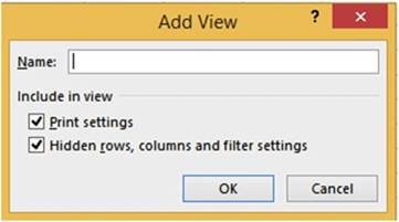
Figure 5-29. The Add View dialog box
After you have created your views you can switch to another view by selecting it from the Custom Views dialog
box and then clicking the Show button.
■
NoteYou can�t create a custom view that contains
a table.
169
CHAPTER 5 ■ DIFFERENT WAYS OF VIEWING AND PRINTING YOUR
WORKBOOK
In this exercise you will create three views, display the views, and
then delete them.
Create
Views
1.
Open workbook Chapter 5 if it isn�t already open.
Click the Custom tab.
2.
Drag across column
heads D, E, F, and G to select them. Right-click the selected text and select Hide.
3.
Click the Ribbon�s
View tab. In the Workbook
Views group click the Custom
Views button.
4.
Click the Add button in the Custom Views window.
Enter Original
View for the name of the custom view as shown in Figure 5-30. Click the OK button.
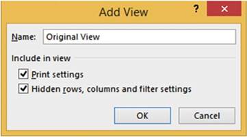
Figure 5-30. Add View window
5.
Drag across column
heads C and H to select them.
Right-click the selected
text and select
Unhide.
6.
Drag across row heads 15 to 20 to select them. Right-click the selected text and select
Hide.
7.
Click the Ribbon�s
View tab. In the Workbook
Views group, click the Custom
Views button.
8.
Click the Add button in the Custom Views window.
9.
Enter Hidden Rows for the name
of the custom view. Click the OK
button.
10.
On the Ribbon�s
Page Layout tab, in the Page Setup group, click
the Orientation button
then select Landscape.
11.
Select the range
A1:K6. Click the Ribbon�s Page
Layout tab; in the Page
Setup group,
click the Print Area button.
Select Set Print Area. In the Sheet Options group,
select Print in the Gridlines
area.
170
CHAPTER 5 ■ DIFFERENT WAYS OF VIEWING AND PRINTING YOUR
WORKBOOK
12.
Click the Page Setup group�s dialog box launcher
 :
:
a.
Click the Sheet tab.
b.
Enter A1:K6 in the Print area text box.
c.
Select Gridlines.
d.
Click the OK button.
13.
Click the Ribbon�s
View tab. In the Workbook
Views group click the Custom
Views button.
14.
In the Custom Views window
click the Add button. Enter
Print Change for the Name in the Add View window.
Click the OK button.
Show a View
1.
Click the Custom Views button.
Click Original View and then click the Show button.
See Figure 5-31 (columns D through
G are hidden).
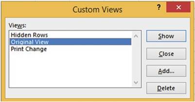
Figure5-31.CustomViewswindow
2.
Click the Custom
Views button. Click
Hidden Rows and then click
the Show button.
Rows 15 through
20 are hidden.
3.
Click the Custom Views button.
Click Print Change
and then click the Show button. Click the Ribbon�s
File tab. Click
Print in the left pane.
You can see that only what you selected for the print
area is going
to print and it is in landscape mode. Click the Return
button.
Delete a
View
1.
In the Workbook Views group click the Custom Views button.
2.
Select a View and then click the Delete button.
You will be asked to confirm the deletion. Click
Yes.
3.
Repeat steps 1 and 2 for the other two views.
171
CHAPTER 5 ■ DIFFERENT WAYS OF VIEWING AND PRINTING YOUR
WORKBOOK
This section
showed you how to create your own custom views so that the same worksheet can
be viewed in different ways.
Each custom view is assigned its own name. All the custom views for the
workbook are stored within the
workbook. If you didn�t use custom views, you would have to save different
versions of the workbook to get the
same result.
Summary
Excel can display a spreadsheet in one of three different views. Normal view is the view you will use most of
the time. Page Break view is useful for adjusting page breaks. Page Layout view provides a quick way to add,
edit, and delete headers and footers.
Custom views allow you or other users to switch back and forth between different views of the same
spreadsheet. An example would be you create one view to show all of your data, a second view to show certain
columns, and a third view to print a portion of a worksheet.
You have split worksheets into multiple panes and then scrolled through the individual panes. You�ve
practiced making the worksheet look the way you want it to and used many of the buttons you can see when you
open Excel. Next, you will be learning about the �Backstage� which includes more options for saving the
workbook in different formats and how to keep track of information about when the workbook was created and
why. You�ll also practice how to share workbooks via e-mail. Other features and tabs discussed next include
how to keep track of your recent work and how to use the navigation pane.
172
CHAPTER
6
Understanding Backstage
The File tab, unlike the other tabs,
doesn�t bring up a series
of groups with buttons on them; rather,
it brings up what is called the Backstage. This area is called the Backstage because
the options on the Backstage are things that are handled
behind the scenes
from the workbook
such as handling
files, printing, sharing
and exporting workbooks, account information, and selecting the options that change how Excel works.
It also displays
information about the workbook.
After reading and working through this
chapter you should be able to
�
Save a workbook in different formats
�
Add and edit information about a file and
its properties
�
Use various options to print the workbook
the way you want it to appear
�
Send a workbook as an e-mail attachment
�
Search for a template that meets your needs
�
Open a workbook
by browsing for it or by using
the Recent list
�
Specify the number of workbooks that appear
in the Recent list
�
Keep workbooks on the Recent list
�
Place recently opened workbooks in the
Navigation pane
�
Set Excel Options
Backstage
Overview
Figure 6-1 shows the Backstage. Clicking a group
item in the Navigation pane such as Info, New, Open, etc., displays information and options
for that grouping
in the area to the right. We will cover
most of the groups
in the Navigation pane.
The list that follows
shows some of the things
that you can do from Backstage:
�
Save files in many different formats
�
Change printer settings
�
Protect the workbook
�
Save the workbook to OneDrive
�
Give others rights to your workbook
173
CHAPTER 6 ■ UNDERSTANDING BACKSTAGE
�
E-mail the workbook in various formats
�
Add and remove personal information from the
workbook
�
Check the accessibility of your workbook for
those with disabilities
�
Check for compatibility with previous Excel
versions
�
Update Excel
�
Change information on your Microsoft Account
�
Specify the number of workbooks that appear
in the Recent list
�
Pin workbooks to the backstage pane
�
Recover unsaved workbooks
Table 6-1 lists some of the groups from the Navigation pane and
describes them.
Table6-1.BackstageNavigationGroupsandTheirDescriptions

Group�� Description
Info��� Displays
information about the currently opened
workbook.
New��� Creates a new blank workbook
or creates a workbook from a template.
Open��� Opens an existing
Excel workbook.
Save��� Saves updates
to the currently open workbook.
Doesn�t change the name of the existing workbook.
Save As��
Saves a workbook
that hasn�t been previously saved. It can also be used to create a second
copy of the currently open workbook and assign it a different
name.
Print��� Prints options for printing the workbook.
Share��� Provides options for sharing your workbook with others.
Close��� Closes the workbook.
Account�� Provides
your Microsoft Office
Account Information.
Options�� Shows options you can set to change
how Excel works.
Info Group�Viewing, Adding, and Editing Information About the
Workbook
The Info group is displayed
by default in the Backstage
when you click the File tab. See Figure 6-1.
■
Note� If you start a new workbook and click the File tab without having
made an entry
into a cell, then your Backstage will display with the Open group selected. Excel assumes that since there
are no entries you want to open a workbook.
The Info group displays
information about the currently open workbook and handles information related to it. We will first look at
the Properties Pane tab; then we will look at the options
in the middle pane for protecting and inspecting the workbook.
174
CHAPTER 6 ■ UNDERSTANDING BACKSTAGE
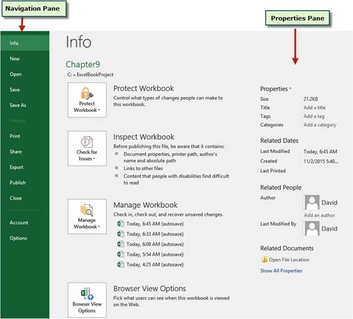
Figure 6-1.Backstage when accessed from a workbook
with data in it
Properties Pane
When you look at a file in Windows Explorer you can see the file�s name, its date, and size, but often this
isn�t enough information. Additional information about the file can be entered or viewed in the Properties
pane, located to the right of the Info pane. At the bottom of the Properties pane you can click
ShowAllProperties if not all of the properties are currently showing. You can click
ShowFewerPropertiesif all properties are currently showing.
You can enter or edit the properties directly
on this window.
You can enter
such things as the title,
tags, categories, Company,
and Manager.
Clicking the down arrow next to Properties in the Properties pane brings up the Advanced
Properties
button shown in Figure 6-2. Clicking
the Advanced Properties button displays
the Properties dialog
box as shown in Figure 6-3.
175
CHAPTER 6 ■ UNDERSTANDING BACKSTAGE
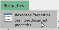
Figure6-2.AdvancedPropertiesbutton
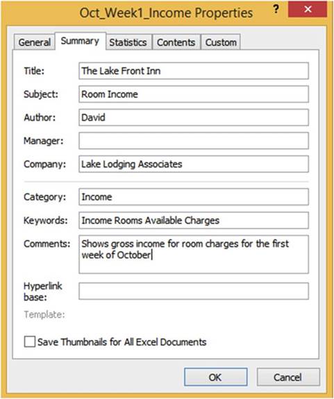
Figure6-3.WorkbookPropertiesdialogbox
Some of the information you enter in the properties dialog box can be viewed in the Properties pane. It
is also displayed at the bottom of the Save As window as shown in Figure 6-4. The information you enter here
is useful as documentation and can help you search for the workbook.
176
CHAPTER 6 ■ UNDERSTANDING BACKSTAGE
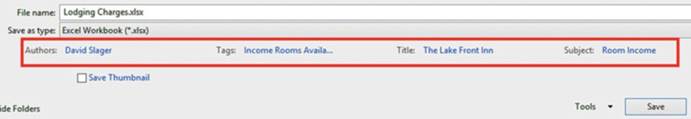
Figure 6-4.Some of the information you enter in the Properties dialog box appears
when you save a file using Save As from the Backstage�s Navigation pane
Right-clicking the file in Windows Explorer
and then selecting Properties displays the Properties window.
Select the Details
tab to see the information you entered. See Figure 6-5.
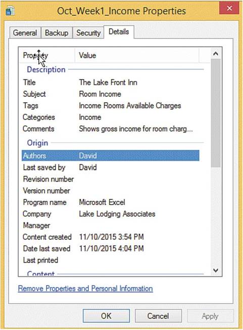
Figure6-5.WorkbookinformationfortheWorkbooknamedOct_Week1_Income
177
CHAPTER 6 ■ UNDERSTANDING BACKSTAGE
Protect Workbook Options
In the Info pane, clicking the Protect Workbook button brings up a menu of options for different ways of
protecting your workbook. See Figure 6-6. We will cover Mark as Final, Encrypt with Password, and Protect
Workbook Structure. These aren�t the only options for protecting your workbook. We look at other ways to
protect your workbook later in this chapter.
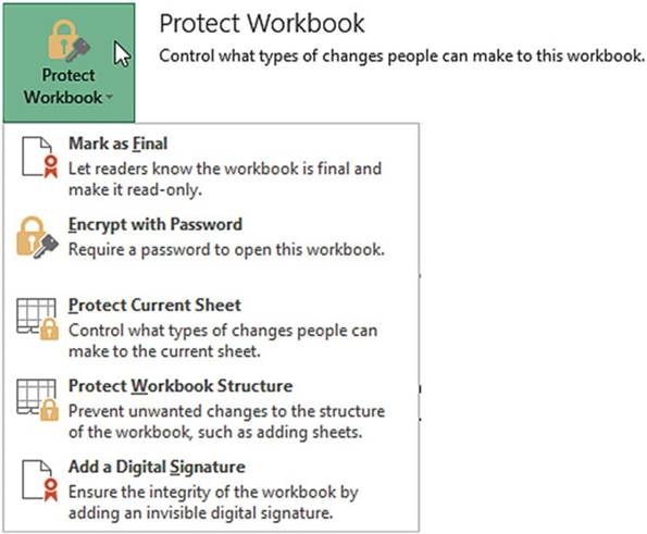
Figure6-6.Optionsforprotectingaworkbook
Mark as Final
Selecting Mark as Final will make your workbook read only. You won�t be able to make any changes to any
worksheet
and you won�t be able to create any new worksheets. Clicking
the Mark as Final button will bring up
the message box shown in Figure 6-7.
178
CHAPTER 6 ■ UNDERSTANDING BACKSTAGE
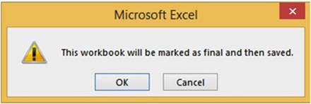
Figure 6-7.Excel asking if you want to mark the
workbook as final
Clicking
the OK button brings up the message
window shown in Figure 6-8.
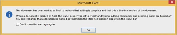
Figure 6-8.Message informing that editing
is complete and this is the final
version
The workbook
opens with a Marked as Final icon on the status bar and a message above the worksheet indicating that
the author has marked the workbook
as final to discourage editing.
See Figure 6-9. If you
or anyone you give this workbook
to decides that a change
is necessary, it can be done by clicking the Edit
Anyway button. Clicking this button
allows you to make any changes or additions to any worksheet
in the workbook.
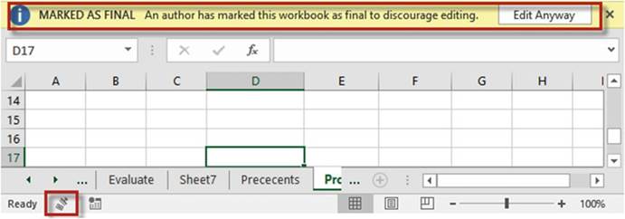
Figure6-9.WorkbookthathasbeenMarkedasFinal
179
CHAPTER 6 ■ UNDERSTANDING BACKSTAGE
Encrypt with Password
Selecting
this option requires
you to enter a password
and then verify
it. It uses 128-bit advanced
encryption to make your file more secure. You will need to use this password
the next time you open the file.
■
Note� Microsoft does not provide a way to recover passwords created in Microsoft
Office.
Protect Workbook Structure
This option prevents
users from adding or deleting
worksheets; hiding and unhiding worksheets; and moving, copying, or renaming worksheets. You can add a
password
to this option if you desire. See Figure 6-10.
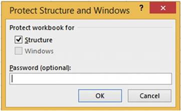
Figure 6-10.Structure protection selected to prevent user from making changes
If password
protection has been applied to the workbook
and if protection for workbook
structure has been applied, the Protect Workbook
area would notify you of this. See Figure 6-11.
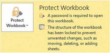
Figure 6-11.Message notifying user that the structure has been locked
and a password is required
to open the workbook
Check
for Issues
Just to the right of the Check
for Issues button
is the Inspect Workbook area.
The Inspect Workbook
shows items that have not been resolved. See Figure 6-12. These
are not problems
that will keep your workbook from working.
180
CHAPTER 6 ■ UNDERSTANDING BACKSTAGE
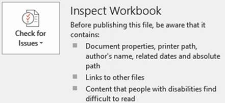
Figure 6-12.Inspect Workbook shows items
that have not been resolved
The Check
for Issues button
has options for checking if the workbook
contains personal information, checking if the workbook
can be easily read by users with disabilities, and checking for compatibility with previous Excel versions.
See Figure 6-13. We will cover
the Inspect Document
and Check Compatibility.
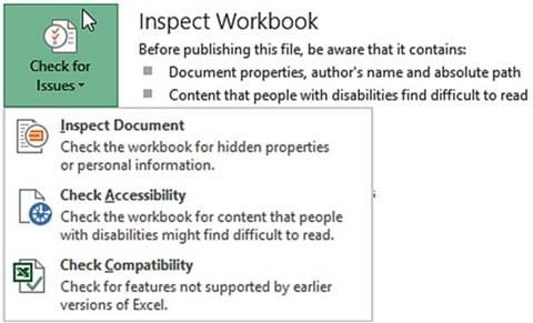
Figure6-13.CheckforIssuesoptions
Inspect Document
The Document Inspector helps you find personal and hidden information that you may want to remove
before sharing this document with anybody else.
If you run Inspect Document
before you have saved your Excel workbook, you will get the warning message
in Figure 6-14 that you should click Yes to save the file now,
otherwise you might
lose some of your data.
181
CHAPTER 6 ■ UNDERSTANDING BACKSTAGE
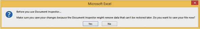
Figure 6-14.Message informing user to click the Yes button
to save the file
If you have already
saved the file or you have responded
to the message in Figure 6-14, then the Document Inspector
dialog box displays.
See Figure 6-15. Check each check box in the Document
Inspector that you want to check.
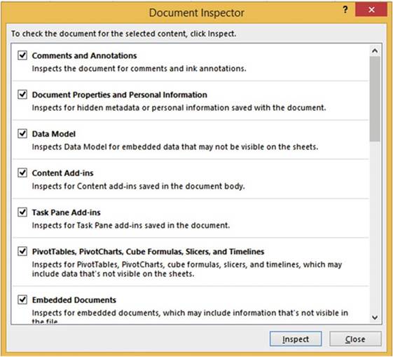
Figure6-15.Selectitemsyouwantinspected
182
CHAPTER 6 ■ UNDERSTANDING BACKSTAGE
Clicking the Inspect button
inspects for those
items that you have checked.
If Excel finds
personal or hidden
data for any option you have selected, it will display
a Remove All button for that option. See Figure 6-16.
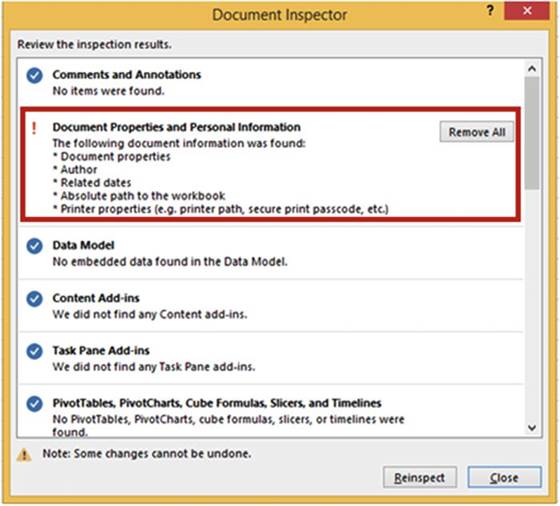
Figure
6-16.Excel reports on personal or hidden data it has found for the options
you selected
183
CHAPTER 6 ■ UNDERSTANDING BACKSTAGE
Check Compatibility
Excel 2016 has capabilities that previous versions
did not. If you want to share a 2016 workbook with someone else who doesn�t
have 2016 you will want to run the Compatibility Checker. The Compatibility Checker gives a report
on what functionality may be lost and how many times that functionality occurs
in the workbook. See Figure 6-17. If you save a workbook
in the Excel 97-2003 format
the Compatibility Checker
will run automatically. Workbooks in the 97-2003 format
have a file extension of .xls. Workbooks
starting with version
2007 have an extension of .xlsx.
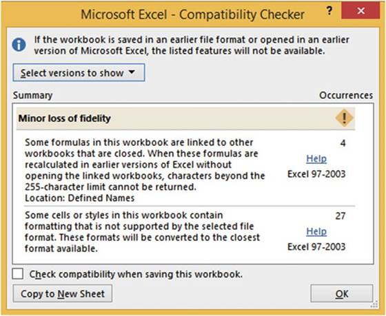
Figure 6-17. Compatibility Checker
184
CHAPTER 6 ■ UNDERSTANDING BACKSTAGE
Clicking the Selectversionstoshowbutton in the Compatibility Checker brings up
the Excel versions to test for. See Figure 6-18. The Compatibility Checker will test for compatibility with
the Excel versions you have selected.
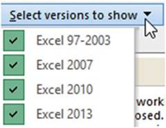
Figure6-18.SelectwhichExcelversionstotestfor
Select the check
box for Check compatibility when saving this workbook to have Excel check
for compatibility each time you save this workbook.
New Group�Creating a New Workbook
You can create a new workbook by clicking New in the Navigation pane of Backstage or by pressing
Ctrl + N while not in Backstage. Selecting New from the Navigation pane allows you to create
a new blank document from scratch,
but if the project you are going
to create is similar to one of the vast number of pre-built templates, you might want to consider
using one of them instead
(see Figure 6-19). As the saying
goes, �No sense in reinventing the wheel.�
185
CHAPTER 6 ■ UNDERSTANDING BACKSTAGE
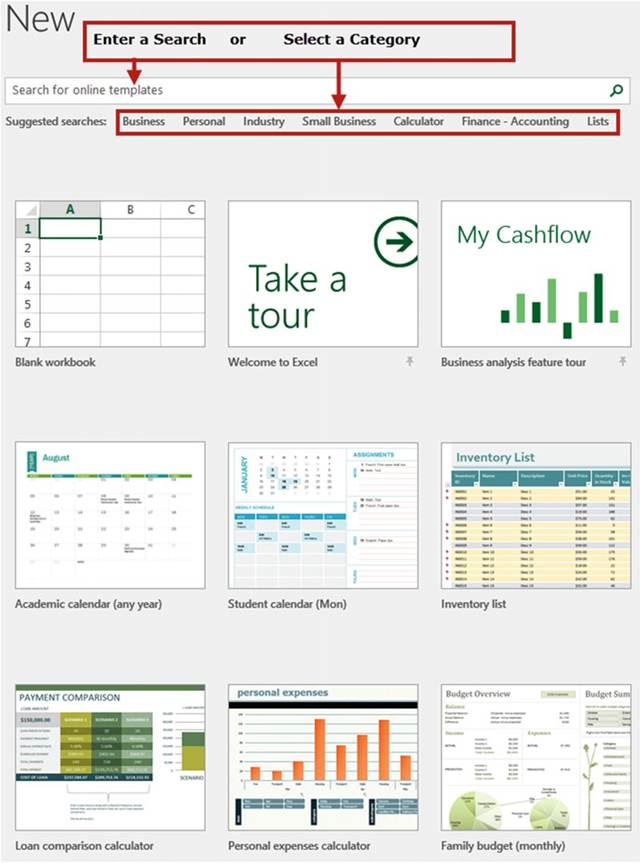
Figure6-19.Searchforatemplateorselectone
186
CHAPTER 6 ■ UNDERSTANDING BACKSTAGE
If you select one of the template categories, Excel displays available templates in that category and
provides other
categories on the right for you to select from.
See Figure 6-20.
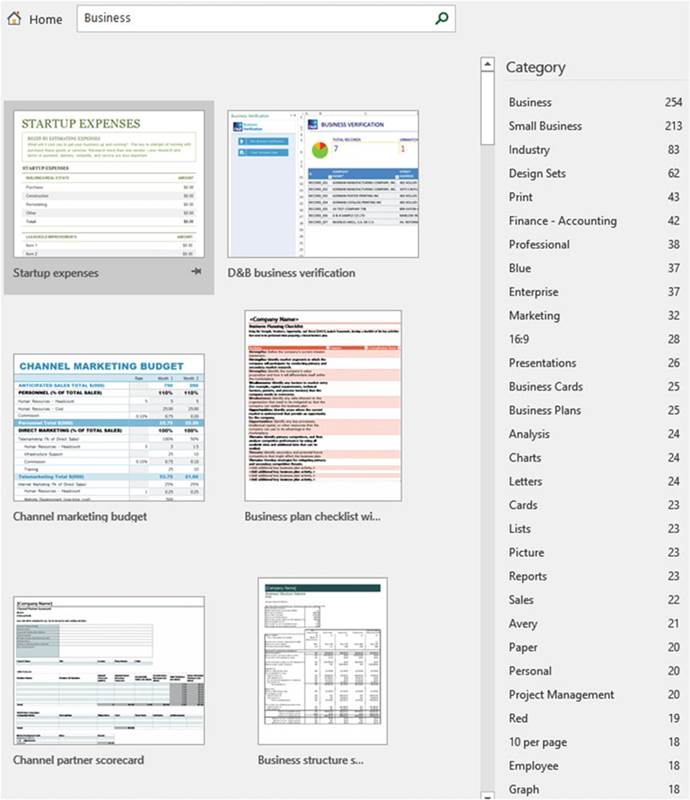
Figure 6-20.Available templates for selected
category on left; additional categories on right side
187
CHAPTER 6 ■ UNDERSTANDING BACKSTAGE
Double-click the template you want to use. Excel
opens a new workbook that uses that template. If you want to see a larger
view of the template before
you open it you can single-click it. See Figure
6-21. You can use the Next and Previous buttons
to view other
templates. You can click the Create button
to open the template.
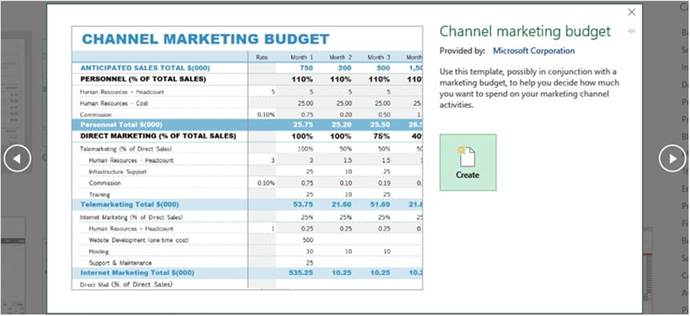
Figure6-21.Single-clickingatemplateshowsanenlargedviewofit
Open Group�Open a Workbook
From the Open group you can browse for a workbook or select it from a Recent list. You can pin a workbook
if you want it to remain in the Recent list.
Opening an Existing Workbook
From the Open group in the Backstage
view you can open a workbook by doing one of the following:
�
Select a workbook from the Recent list
�
Select a location
of an Excel file such as OneDrive
or a web location.
�
Select PC to find an Excel file on your local computer or network. You may need to
click the Browse button to get to the workbook
file location.
Opening a Workbook
from the Recent
List
If you used the workbook
recently it would be easier to open the file by selecting
Recent in the middle pane. Selecting Recent displays a list of the workbooks
that you have opened recently.
The most recent one would be
at the top of the list. Excel breaks it down into workbooks you used Today, Yesterday, This Week, Last Week,
and Older. Excel shows the file name, its path, and to the right of that the date and time it was saved.
See Figure 6-22.
188
CHAPTER 6 ■ UNDERSTANDING BACKSTAGE
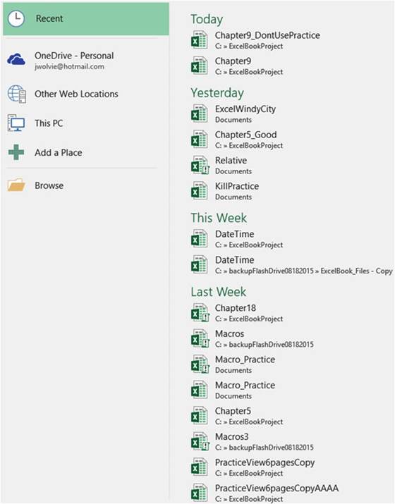
Figure 6-22.Recently used workbooks and where they are stored
If the workbook
you need to open isn�t
in the Recent list, you can use one of the other
options such as accessing workbooks from OneDrive or other locations on your PC.
Keeping Workbooks on the Recent
List
When you move your mouse cursor over a workbook
name in the Recent list in the Backstage you see a pin to the right of the workbook name. See Figure 6-23.
189
CHAPTER 6 ■ UNDERSTANDING BACKSTAGE

Figure 6-23. Pins
Clicking a pin will change the pin view from horizontal to vertical
 . When the pin displays
vertically, the workbook
associated with that pin will remain on the Recent
list no matter
how many files
you open and close. Pinned
items are displayed at the top of the Recent list.
See Figure 6-24. You can unpin
the workbook by clicking the pin again.
. When the pin displays
vertically, the workbook
associated with that pin will remain on the Recent
list no matter
how many files
you open and close. Pinned
items are displayed at the top of the Recent list.
See Figure 6-24. You can unpin
the workbook by clicking the pin again.
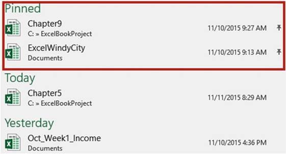
Figure6-24.PinnedworkbooksstayatthetopoftheRecentlist
Right-clicking a workbook in the Recent
list brings up a context
menu with six options, including Pin to list, which
works the same way that clicking the pin next to the file does.
See Figure 6-25.
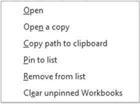
Figure6-25.Contextmenuwithsixoptions
190
CHAPTER 6 ■ UNDERSTANDING BACKSTAGE
In addition to pinning or unpinning a workbook from this menu, you also can choose to
�
Open the workbook.
�
Open a copy of the workbook which keeps your
original protected.
�
Copy path to clipboard�copies the path and the file name to the clipboard from where you can paste
it into a worksheet.
�
Remove the workbook from the Recent list.
�
Remove all workbooks from the Recent list
that are not pinned.
Options
Affecting the Open Group
There are two options that you can set in the Options
group that affect
how many workbooks appear in the Recent list and how many will appear on another available list on the
Navigation pane.
Specifying the Number of Workbooks That
Appear in the Recent List
How many workbooks appear in the recent list depends upon how many are specified in the Excel
Options window. By default,
the list shows
the 25 most recent workbooks, but you can adjust that number higher
or lower. To change the number that appear in the list click the File tab on the Ribbon, click
Options in the Navigation pane, and then click Advanced
in the left pane. You will have to scroll
down to find the Display
section. Change Show this number of Recent Workbooks
to whatever
you want. See Figure 6-26. Click
the OK button.
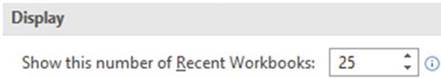
Figure 6-26.Select
the number of recent documents
to display in Backstage
Placing Recently Opened Workbooks in the
Navigation Pane
If you want even quicker
access to your workbooks, select the next option in the Display
section. Checking Quickly access the number of Recent Workbooks
places the number of workbooks that you specify
on the Navigation Pane. See Figure 6-27.
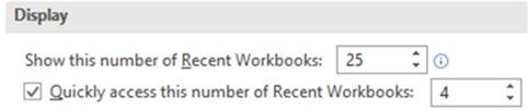
Figure 6-27.Checking the Quickly
access option displays
the number you entered of the latest
used workbooks on the Navigation pane
Figure 6-28 displays an example
of how the Navigation pane looks when four workbooks
are selected for quick access.
These four workbooks
will remain on the Navigation pane. Clicking one of these workbooks
will open it.
191
CHAPTER 6 ■ UNDERSTANDING BACKSTAGE
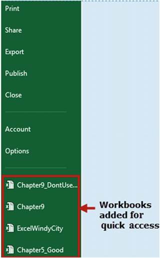
Figure6-28.Thefourlatestworkbooksused
Save and Save As groups�Saving a Workbook
Using Save or Save As
While you are working in Excel everything that you create and import such as your data, charts, graphics,
and so on are all stored in the computer�s random access memory (RAM). Your RAM is only temporary
storage. When you shut off your computer
everything in RAM is cleared.
This is why if something
happens to your computer
or if the power goes off you will lose all the additions and changes you have made since your last save.
Additions and changes are not saved to your hard drive or other type of permanent storage
until you perform
a Save. When you save the workbook
the information is taken from your RAM and stored in a file on your permanent
storage.
If something goes wrong, such as the power going out, and you haven�t
saved your work for quite
some time, don�t panic
because Excel may have already
saved your work to your permanent storage
device using the AutoRecover feature
which we will look at later in this chapter.
There are two backstage groups dedicated to saving a workbook: the Save group
and the Save As group.
Actually, Save isn�t much of a group because it contains no options. The Save As group is almost identical
to the Open group which you have already seen earlier in this chapter. If you click the Save group
and the
workbook has previously been saved then Excel updates
the workbook with your most recent changes.
If you select Save and this is the first time you are saving the workbook, Excel opens the Save As window
(this works the same as if you had clicked
Save As).
192
CHAPTER 6 ■ UNDERSTANDING BACKSTAGE
In the Save As window you must select
a folder where
the workbook will be saved.
Next, you need to enter
the file name for the workbook file.
Excel uses the file name Book1 by default. You will want to
change the name to something that matches with what type of data the workbook contains; for example, if the
workbook contains your Inventory as of June 30, 2011 then name it something like �Inventory_063011.� Next,
you will need to select the Saveastypefor the file you are saving. The default file
type for Workbooks is ExcelWorkbook. This is the format you will probably use most often. If
you want to use a different format you can click the down arrow for the Save As type. As you can see in
Figure 6-29 the workbook can be saved in a lot of different formats.
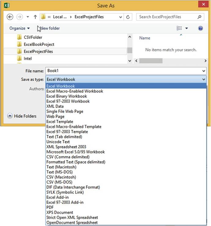
Figure 6-29.You can save the file in one of many different file types
193
CHAPTER 6 ■ UNDERSTANDING BACKSTAGE
Excel automatically adds an extension to your file based on the file type that you have selected. If you had
entered Inventory_063011 for the file name, your complete file name would
be
Inventory_063011.xlsx. Windows explorer
uses these types to determine
what icon to display next to the file
name.
The file name along
with the path can be a maximum
of 255 characters. The path is the drive and folders you need to go through
to get to your file.
An example would
be C:\users\Annette\My Documents\ Inventory_063011.xlsx. You can use spaces in the file name but it
is better to use an underscore to� separate words. The following characters can�t be used in a file name:
< > (angle
brackets), | (pipe symbol)
\ (backslash), ? (question mark),
: (colon), * (asterisk), �"
(quotation marks).
An alternative to saving the workbook to your computer
is to store the workbook
online using OneDrive.
OneDrive is an online storage area provided for free from Microsoft. See Figure 6-30. Clicking
OneDrive brings up a Save As window just like when you save files to your personal
computer or network.
You can create folders in OneDrive just like you can on your hard drive.
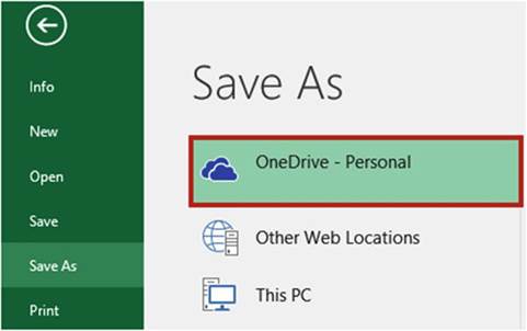
Figure 6-30. Save file to OneDrive
Document Recovery
You should save your workbook
often, but if you haven�t
done a save and your system crashes
or you suddenly lose power, don�t
panic. Excel has a feature
called AutoRecover which
automatically saves your file
at the interval you specify.
The interval can be set between 1 and 120 minutes. The default time interval is
10 minutes. See Figure 6-30. I like to set mine at 5 minutes or less because
I can make a lot of changes
within that time that I wouldn�t want to lose. Shortening the time might slow down your computer
depending upon the size of the file and number of changes made.
Clicking Options
in the Navigation pane of the Backstage
view brings up the Excel Options window.
See Figure 6-31.
194
CHAPTER 6 ■ UNDERSTANDING BACKSTAGE
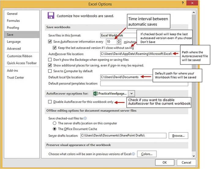
Figure6-31.ExcelOptionswindowwithSavetabselected
Clicking Save in the left pane of the Excel Options
window displays the options for saving workbooks
and using AutoRecover. Here you can set the time interval
between saves, the path where the AutoRecover files will be stored,
if you want to keep the last autosaved version
if you closed without saving,
whether or not you
want to disable AutoRecover for the current
workbook, and so on.
Using the default time interval of 10 minutes,
if you save your Excel
workbook and then 29 minutes
later the power goes out, you will have lost only the changes
that you made during the last 9 minutes because
Excel would have backed up your file at 10 and 20 minutes. When you reopen
the file later,
Excel will display
the Document Recovery
pane containing the Autosaved version
of the file and the original version
of the file.
195
CHAPTER 6 ■ UNDERSTANDING BACKSTAGE
Closed a Workbook Without Saving
If you close a workbook
without saving it and later decide that you really did need to save it, you may still be able to get back
some or all of the changes depending
upon what you set the AutoRecover time interval for and
how much time elapsed since your last save.
If you close your Excel workbook and you haven�t
saved it and any changes
you have made to it have
been done during the AutoRecover time interval, Excel will display
the message in Figure 6-32.
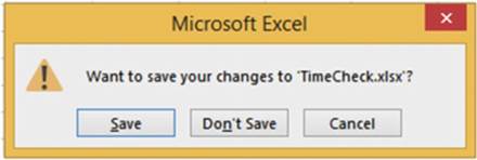
Figure6-32.Warningthatyouareclosingtheworkbookbeforesavingit
If you click Don�t Save, your changes will be lost.
If you close your Excel workbook and you haven�t
saved it and you have made changes
to it after the time interval
you set for AutoRecover, Excel will display
the message in Figure 6-33.
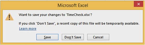
Figure 6-33.Message that if choose not to save the file a temporary one will still be
available
196
CHAPTER 6 ■ UNDERSTANDING BACKSTAGE
If you click Don�t
Save you can recover at least some of the changes you made.
If there are no other workbooks
open when you start Excel and there are files that Excel has recovered, you will see the pane in Figure
6-34.
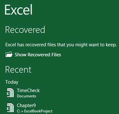
Figure6-34.Youcanchoosetoshowanyrecoveredfiles
Clicking ShowRecoveredFilesbrings up the files that Excel has recovered. See Figure
6-35.
197
CHAPTER 6 ■ UNDERSTANDING BACKSTAGE
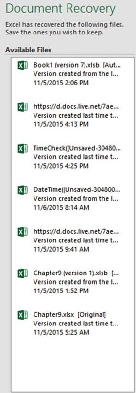
Figure6-35.Recoveredfilesthatyoucansave
Clicking any of the recovered files in Figure
6-35 displays a drop-down arrow. Clicking the drop-down arrow displays a context menu from which you can
select Open, Save As, or Delete, or Show Repairs.
See Figure 6-36.
198
CHAPTER 6 ■ UNDERSTANDING BACKSTAGE
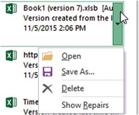
Figure6-36.Optionsforrecoveredfiles
Selecting Show Repairs will open the file and display a message if the file contains any errors and if any
repairs were made to the file.
If you close Excel and have not deleted the Autosaved files, Excel will ask if you want to view the files
later or remove them. See Figure
6-37. If you select �Yes, I want to view these files later,� Excel will keep the
files and display them in the Document
Recovery pane the next time you start Excel.
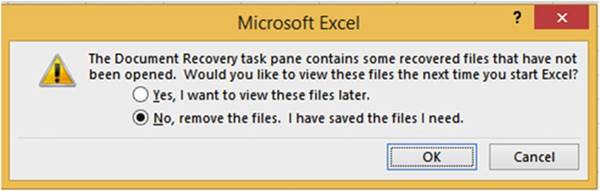
Figure 6-37.Message asking if you want to view the recovered files
later or if you want to remove
them
If you open a workbook that has unsaved
changes, Excel will display a message next to the Manage
Workbook button. See Figure 6-38.
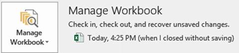
Figure 6-38.Message when opening a workbook that was closed
without being saved
Click the Manage Workbook
button to see if there are any other recoverable unsaved workbooks. See Figure 6-39.
199
CHAPTER 6 ■ UNDERSTANDING BACKSTAGE
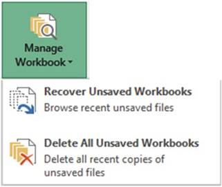
Figure 6-39. Manage Workbook button
Click Recover Unsaved
Workbooks. The Open dialog box displays showing
any unsaved files. The file displays the workbook�s name followed by a long number. See Figure 6-40.

Figure6-40.Unsavedfileshavealongnumberaddedtotheirname
Double-clicking the Unsaved file opens the file in Excel. You will see the message
shown in Figure
6-41.
Click Save As and assign the workbook a new
name.
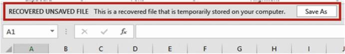
Figure6-41.RecoveredUnsavedFilemessage
■
Note� You should recover
any unsaved file immediately after
you realize it wasn�t saved
because these unsaved
files are only kept temporarily.
200
CHAPTER 6 ■ UNDERSTANDING BACKSTAGE
Saving Workbooks
with Protections: Backups
and Limiting Changes
You can set a password
at the file level to prevent an unauthorized user from opening
a workbook. You can also allow a user to open the workbook but not save any changes,
except as a new file. In this section,
we�ll see how to set up regular
backups for your workbooks, protect
the original file using Read Only, and password-protect your workbooks.
With the workbook
you want protected
open, and click the Ribbon�s
File tab. Click Save As in the Navigation pane. In the Save As dialog box, click the Tools drop-down
menu and select General Options.
See Figure 6-42.
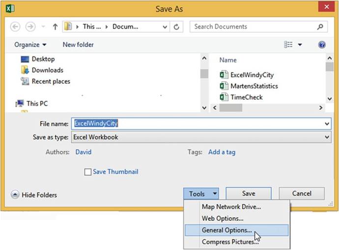
Figure6-42.ToolsoptionsintheSaveAsdialogbox
The General Options
dialog box opens. Click the check box for Always create backup. This will create a backup file of the
file you are saving in the same location.
The file will be named Backup of followed by the name you give the workbook. It will be given an
extension of .xlk. For example, if you name your file Invoices.xlsx, the backup file will be
named Backup of Invoices.xlk. See Figure 6-43.
201
CHAPTER 6 ■ UNDERSTANDING BACKSTAGE
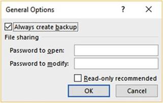
Figure 6-43.General Options with Always
create backup selected
When you save your file the first
time after having
selected Always create backup, only the original
file will save,
there will not be a backup. Let�s
say you only entered a value in cell A1 and you name the file
Invoices.xlsx. Now you add to the worksheet
by entering a value in cell B1 and save the workbook
again. The
Invoices.xlsx file now contains values in cell A1 and B1, a backup is created named Backup of
Invoices.xlk
which only contains the value in cell A1. Let�s do one more.
You add a value in cell c3 in the Invoices.xlsxworkbook and save the file again. Now the
Invoices.xlsx file contains values in cells A1, B1, and C1 but the backup file
BackupofInvoices.xlkonly contains values in cells A1 and B1. The backup file stays one
generation (copy) behind.
Check the check box for Read-onlyrecommendedif you want to give the user the capability to view
the workbook but not make any changes.
You can require that the user enter a password for both
the Password to open
and Password to modify,
either one or neither.
Remember, if you forget your password you can�t get it back.
Enter a password in the Password
to open text box if you want to require
that the user enter this password before opening the workbook. The user can view or change the workbook.
Enter a second password
in the Password
to modify text box if you want to require
that the user enter
this password
if he or she wants
to modify the workbook. The user will be able to view the workbook
as read only if he doesn�t enter
the password.
You should enter both passwords if you want to require
that the user enter a password to open the workbook and then require
them to enter a second one to modify the workbook. The passwords should not
be the same.
If you entered a password for Password to open you will need to confirm
that password. See Figure 6-44.
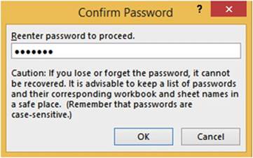
Figure 6-44.Confirm password if you entered a password for Password to open
202
CHAPTER 6 ■ UNDERSTANDING BACKSTAGE
If you entered
a password for Password to modify you will need to confirm
that password. See Figure 6-45.
If you entered
both passwords you will be required to confirm both of them.
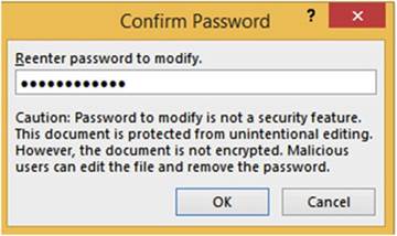
Figure 6-45.Confirm password if you entered a password for Password to modify
Clicking the Save button saves the workbook with the options
you entered for General Options.
See Figure 6-46.
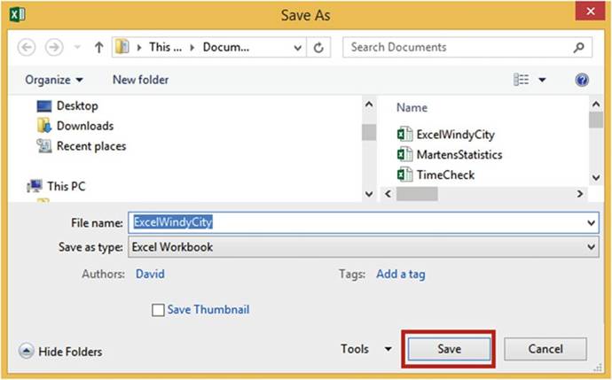
Figure6-46.Savethefileusingtheselectionsyoumade
203
CHAPTER 6 ■ UNDERSTANDING BACKSTAGE
If you entered passwords, you will be required to enter them once you have closed
the workbook and reopened it.
�
If you required a password to open the workbook you will see the window
in Figure 6-47 when opening
the workbook.
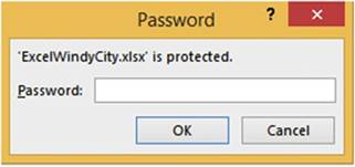
Figure6-47.Passwordrequiredtoopenworkbook
�
If you required a password for modifying the workbook, another
Password window opens. The user must enter a password in order to modify the workbook. She can open the
workbook
in Read Only without entering
a password by clicking the Read
Only button. See Figure 6-48.
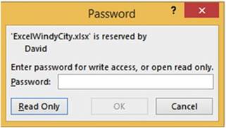
Figure 6-48.Enter password to modify workbook or
click Read Only button
If the user clicks the Read Only button,
he can make changes to the workbook
but when he tries to save
it, he will not be able to, thus preventing any changes from being made. The user will get the message
in Figure 6-49.
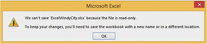
Figure
6-49.Messagesayingthefileisread-only.Ifyouwanttosavechangesyouwillneedtosavethefile
withanewname
204
CHAPTER 6 ■ UNDERSTANDING BACKSTAGE
If a password is required to open the workbook and the user elected to use Read Only instead
of entering the password
for modifying, the Backstage will show as in Figure
6-50.
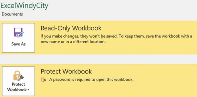
Figure6-50.Backstagemessages
Print Group�Printing a Workbook
The left pane of the Print group (Figure 6-51) contains
Settings for controlling how the worksheet
or workbook is to be printed.
Many of these same options
are available on the Page Layout tab on the ribbon.
The right pane of the Print group displays what the current
document will look like when it is printed based on the print options
used in the left pane.
205
CHAPTER 6 ■ UNDERSTANDING BACKSTAGE
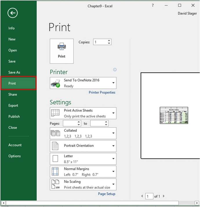
Figure 6-51. Printing options
You should first make any necessary
changes to the Printer and Settings properties
and then click the
Print button to actually do the printing.
Selecting a Printer
One of the decisions you will need to make is where
you want your report printed
to. You don�t
have to print to
a printer. You can print
to programs, to other devices
such as a fax machine,
or to a file. Clicking
the down arrow for the printer lists
all your currently available options. See Figure 6-52. What appears here depends upon what programs
you have and what you have attached
to your computer. If the printer
you wish to print
to isn�t in the list but is attached to your computer
or network, click
the Add Printer
option.
206
CHAPTER 6 ■ UNDERSTANDING BACKSTAGE
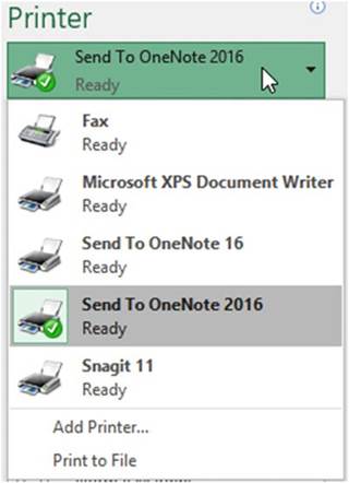
Figure6-52.Locationstowhichtosendyourprinteddata
Printer Settings
The Printer Properties lets you select either landscape
or portrait. The Advanced button in the Printer
Properties gives options
for the paper size and whether you want your graphic images to print at 600 or 1200 dpi.
Selecting to Print Active Worksheets, an
Entire Workbook, or a Selected Portion
The first option in the Settings area is for selecting whether
you want to print only the current
worksheet, the Entire Workbook,
or just the area that you have selected. See Figure 6-53. What you select here is reflected in the right
pane. The Print Active Sheets only prints those worksheets that you currently
have selected. The Print Selection
prints the cells that you currently
have selected.
207
CHAPTER 6 ■ UNDERSTANDING BACKSTAGE
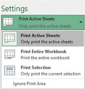
Figure 6-53. Print options
Selecting Which Pages to Print
The next Settings
option lets you select what pages you want to print. The entries in Figure 6-54 will print only pages 2, 3,
and 4. This is true even if you have selected Print Entire Workbook

Figure6-54.Enterthepagerangeyouwanttoprint
Collating
Collating
in Excel works just like collating on a copy machine. If you are printing a worksheet that is five pages and
you select to print four copies,
then selecting Collated will give you four sets of pages 1 through
5. Selecting Uncollated will print four copies of page 1, then four copies of page 2, then four
copies of page 3, and so on. See Figure 6-55.
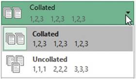
Figure 6-55. Collating options
208
Orientation
CHAPTER 6 ■ UNDERSTANDING BACKSTAGE
You can print in a vertical
format (Portrait) or a horizontal format (Landscape). Selecting Landscape is one way
of printing more columns on a page.
Selecting
Paper Size
You will probably
be printing on letter size (8.5� x 11�) paper,
but if not, you can select another
paper size. See Figure 6-56. If you have a spreadsheet with a lot of columns
you might try using legal
size paper. Excel will automatically adjust your spreadsheet to reflect the selected paper
size.
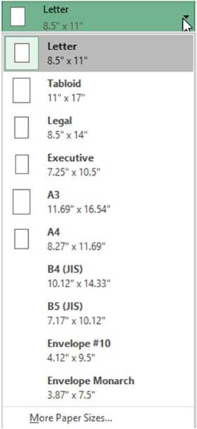
Figure 6-56. Select output size
209
CHAPTER 6 ■ UNDERSTANDING BACKSTAGE
Setting Page Margins
You can use one of Excel�s preset margins for Normal, Wide, or Narrow or you can create your own custom
margins by selecting CustomMargins. See Figure 6-57.
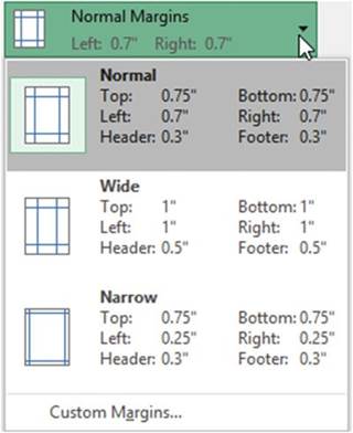
Figure 6-57. Select margins
Clicking Custom Margins
brings up the Page Setup window with the Margins Tab selected. See Figure 6-58.
210
CHAPTER 6 ■ UNDERSTANDING BACKSTAGE
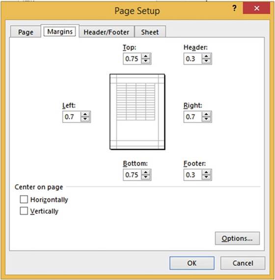
Figure 6-58.Enter
margins and how you want the data centered on the page
The Margins
tab has options for setting
the top, left, right, and bottom margins
of your page as well as setting margins for the header and footers.
You can use the check boxes to specify how you want the data centered on the page. When you select
 �Horizontally,
Vertically,
or both, the image in the middle of the tab will reflect your choices by showing how your data will be
displayed on the report.
�Horizontally,
Vertically,
or both, the image in the middle of the tab will reflect your choices by showing how your data will be
displayed on the report.
Selecting Scaling Options
You can print the report
at its actual size or you can select one of Excel�s
preset Scaling options
that shrink the text and objects
on the report. See Figure
6-59.
211
CHAPTER 6 ■ UNDERSTANDING BACKSTAGE
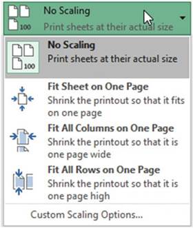
Figure 6-59. Select a Scaling
option
When you are printing a report you probably don�t want to have an extra page for a couple of extra columns
or a few extra rows. This can make reading
your data very difficult. As discussed previously, if there are too many columns to fit on a single page you
could try switching to landscape mode. It will often be easier if you shrink the text and objects
on a worksheet so that they fit on a single paper.
�
Selecting Fit Sheet on One Page will print
everything that is on one worksheet on a single page.
�
Selecting Fit All Columns on One Page shrinks the printout so that it is one page wide, but
your report may print vertically on more than one page.
�
Selecting Fit All Rows on One Page shrinks the
printout so that it is one page high but
your report may print horizontally on more than one page.
�
If none of these options meet your needs you can select Custom Scaling Options. Selecting
Custom Scaling
Options brings up the Page Setup dialog box with the Page tab
selected. See Figure 6-60.
212
CHAPTER 6 ■ UNDERSTANDING BACKSTAGE
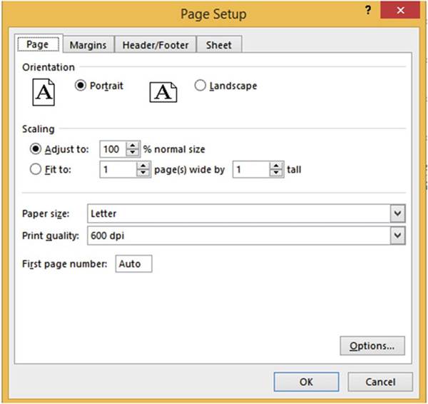
Figure 6-60. Custom Scaling
options
The scaling options here allow you to set the percentage of the actual size you want your report to be.
The value you enter must be between 10 and
400 inclusive.
You can also specify how many pages wide by
how many pages high you want the report.
■
Note� The Page Setup option is located at the bottom of the Settings area in the
Backstage. Clicking Page Setup brings up the Page Setup dialog box. This is the same Page Setup window you
see when you
click
Custom Margins or Custom Scaling options. The Page Setup window includes some of the same options
available in other areas of the Print panel plus some additional options. The Page Setup window can also be
accessed from the Print Layout tab on the Ribbon.
Share
Group�Sharing Workbooks
The Share group
enables you to share workbooks with others. You have multiple
options, including sharing files that you have saved to OneDrive and sending files
via e-mail.
213
CHAPTER 6 ■ UNDERSTANDING BACKSTAGE
Sharing Online with
OneDrive
After you have saved a workbook to your OneDrive, click Share in the Backstage left panel. This brings up the
Share panel in Figure 6-61.

Figure 6-61. Sharing options
Now that you have saved your workbook on OneDrive you can invite others to just view your workbook on
OneDrive or you can let them make changes to it. Right-click the SharewithPeoplebutton
in the right panel shown in Figure 6-61. This brings up the Share window shown in Figure 6-62. Enter the
e-mail address of those people you want to invite to use your workbook. You can select
CanEditor CanView. You can add a message. Click the Share button to send the
e-mails.
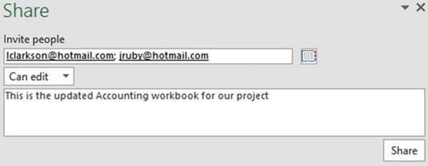
Figure6-62.Invitingotherstoshareyourworkbook
You can also share a workbook
by providing a link to your workbook.
At the bottom of the Share window
you will see Get a sharing link. See Figure 6-63. Click the text link.
214
CHAPTER 6 ■ UNDERSTANDING BACKSTAGE

Figure6-63.ClickthetextGetasharinglink
The window in Figure 6-64 displays. You can click the Createaneditlinkbutton if
you want to provide a user with the ability to edit your workbook online or you can click the
Createaview-onlylinkbutton to provide a user with the ability to only view your
workbook online.
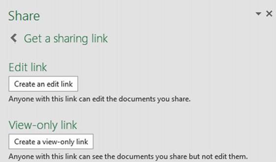
Figure 6-64.Select if you want the user only to be able to view the workbook or if
you want to allow him to
edit it
Figure 6-65 shows the link that was provided
when Create an edit link was clicked.
215
CHAPTER 6 ■ UNDERSTANDING BACKSTAGE
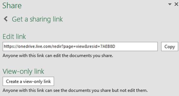
Figure6-65.Provideuserwithlinktoedittheworkbook
You can e-mail
this link to others, you can tell others what it is, you can post it on a web site,
and so on.
Click the arrow to the left of Get a sharing link in Figure 6-65. The Share window
now displays those people to whom you have sent an e-mail
and what rights
you gave them.
It also shows
that you now have an edit link that you can share
with anyone. See Figure 6-66.
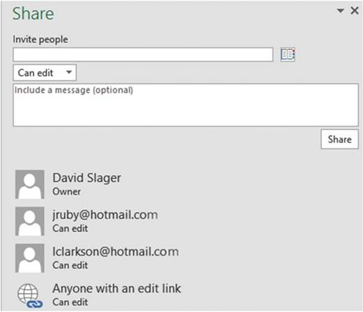
Figure 6-66.Share
window displays with users to whom you have sent an e-mail
216
Sharing
Files Using E-mail
CHAPTER 6 ■ UNDERSTANDING BACKSTAGE
You can send your Excel
workbook to others
in any of the available formats as an e-mail attachment. See Figure 6-67. Those
people receiving your e-mail can then open it in their copy of Excel.

Figure6-67.Selecttheformatyouwanttheworkbooke-mailedin
Clicking the Send as Attachment button brings up Outlook (provided
that you have a copy of Outlook)
with the Excel workbook file already set as the attachment. See Figure 6-68. The Subject is filled
with the name of the Excel workbook.
You can then fill in the e-mail address of the person you are sending it to and perhaps a text message.
Then click the Send button to send the attachment to that e-mail address.
217
CHAPTER 6 ■ UNDERSTANDING BACKSTAGE
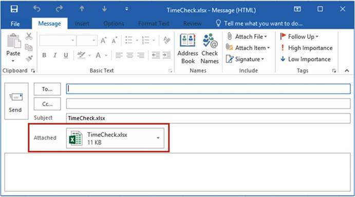
Figure6-68.TheworkbookissetasanattachedfileinOutlook
If the recipient
of your e-mail doesn�t need to edit the workbook
or doesn�t have a copy of Excel, then you can send him or her your workbook in Adobe�s PDF format or
Microsoft�s XPS format. The advantage of sending a file in either one of these formats is that they have
many viewing options
and they don�t require the recipient to have the Excel program.
Account Group
Changes in your Account pane affect all of your Microsoft Office products. Here you can manage your Microsoft
Office Account, check for Microsoft
updates, and change your Office theme. You can also add an Office background pattern that appears
on your title
bar.
Summary
In this chapter
you learned how to use the Backstage
options to manage,
edit, save, and print the workbook.
You also went through protecting your workbooks, recovering them, and sharing
them.
The next chapter shows you how to create formulas manually
or by using a wizard.
Excel functions are built-in formulas.
Functions are what turns Excel into a computational power house rather than just a tool that
allows data entry that you can nicely format and print.
218
CHAPTER 7
Creating and Using Formulas
Formulas are created to
give us the results from such things as adding the items we buy at the store, computing
our taxes, computing our car�s miles per gallon, and so on. A formula in Excel
is an expression that is computed and the results are placed in the
cell that contains the formula. You can enter your own formulas
or you can use of one Excel�s many built-in formulas. Excel�s built-in formulas
are called functions.
After reading
and working through
this chapter you should be able to
�
Enter formulas into a cell or into the formula
bar
�
Enter formulas using
the correct order
of precedence
�
Copy formulas
�
Use the Auto functions
�
View all of the formulas on a worksheet
�
Select named ranges to use in formulas
�
Use absolute and mixed cell references
�
Create and edit named ranges and constants
Formulas
Without the capability to enter formulas, Excel would merely
serve as a sheet for data entry
where you could align
and format data and create
graphs. Excel has formulas for totaling rows and columns,
but Excel allows you
to go way beyond that. You can use one of Excel�s
built-in formulas or you can enter just about any formula you can think
of. You can use very basic formulas
or those that are extremely complex. If you want� to solve the area of a triangle, you can enter
the formula. Do you need to solve
something using the quadratic equation? You can enter
the formula for it.
Introducing Formulas
An example of a formula would be = 5 * 6. The expression returns a value of 30. Formulas always start with
an equal sign (=). Table 7-1 lists math symbols used by Excel and their meanings.
� David Slager 2016
D. Slager, Essential Excel 2016, DOI 10.1007/978-1-4842-2161-7_7
219
CHAPTER 7 ■ CREATING AND USING
FORMULAS
Table7-1.MathSymbolsUsedbyExcel

Symbols for Math Operations
Symbol��� Meaning
+������� Addition
-������ Subtraction
*������ Multiplication
/������ Division
%������ Percent (Converts the
whole number to a Percent)
^����� Exponentiation Ex.(3^2)
=������ Equal to
<������ Less than
<=������ Less than or Equal to
>������ Greater than
>=����� Greater than or Equal
to
<>������ Not
Equal to
Formulas can include specific
values and cell addresses. When a cell address is included in a formula, it is not the address that is used
in the formula but, rather, the value that is in that cell. The result of the expression is placed in the
cell that contains the formula.
If I wanted to add the values in cell A3 and B3 and I wanted the result to be placed in cell C3 I would enter
the formula as shown in Figure 7-1
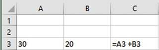
Figure 7-1.Cell
C3 contains the formula for adding the values in cells A3 and B3
Figure 7-2 shows the result
of entering the formula in Figure 7-1.
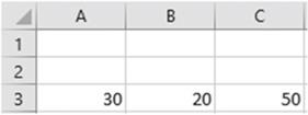
Figure 7-2.Cell
C3 contains the result of adding cells
A3 and B3
220
CHAPTER 7 ■ CREATING AND USING
FORMULAS
If there is a
formula in the current cell. The results of the formula are displayed in the
cell, but the formula is displayed in the formula bar. See Figure 7-3.
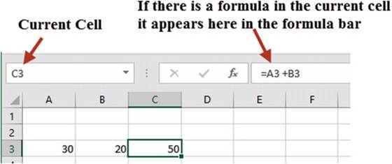
Figure7-3.TheformulaforcellC3appearsinformulabar
Table 7-2 shows examples of formulas and the results they would produce if cell A3 contains a value of 30 and
cell B3 contains a value of 20.
Table 7-2.Excel
Formulas and Their Results (the results would be placed in the cell that contains the formula)


Cell A3
contains a value of 30 Cell B3 contains a value of 20
Entering an = sign as the first character in a cell tells Excel that what follows is a formula.
Entering Formulas
Formulas can be entered
in one of three ways:
�
Typing it directly into a cell
�
Clicking the cells
you want to reference in the formula
separated by mathematical symbols
221
CHAPTER 7 ■ CREATING AND USING
FORMULAS
�
Using your arrow
keys to select
the cells you want to reference separated by mathematical symbols
Typing the Formula
into a Cell
When typing the complete
formula, you start by typing an equal sign then entering any values or cell references that would be
separated by
mathematical symbols. If you enter any cell references in the formula, Excel will
highlight the cell address in the formula and it will place a border around the
cell being referenced. It will highlight both of these in the same color.
The example in Figure 7-4 shows the formula you would enter in cell C1 to add the
values in cells A1 and
B1. When entering A1 in the formula the background color of cell A1 and the
text A1 will be the same color. Cell B2 will have a different matching color for its cell
background and the text B1.
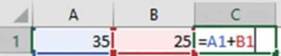
Figure 7-4.Colors
are used to show which
cell is used for which
operand
Creating the Formula by Clicking the Cells You Want to
Reference
Creating formulas by clicking the cells you want to reference is done by first entering an equal sign and
then
clicking any cells you want to reference separated by mathematical symbols.
Using
Figure 7-4 as an example, you would
do the following:
1.
Click inside cell C1
2.
Type the equal sign
3.
Click cell A1 (Excel
enters A1 into the formula)
4.
Type the plus sign
5.
Click cell B1 (Excel
enters B1 into the formula)
6.
Press Enter
Your
formula would be the same as if you had entered it manually =A1+B1.
Creating the Formula Using Your Arrow Keys
The benefit of using your arrow keys to enter a formula is that your hands never have to leave the keyboard.
Using the same example, you would create the formula by doing the following:
1.
Click inside cell C1
2.
Type an equal sign
3.
Press the left arrow key twice to select cell A1
222
CHAPTER 7 ■ CREATING AND USING
FORMULAS
4.
Type a plus sign
5.
Press the left arrow
key once to select cell B1
6.
Press Enter
In this exercise you will enter four formulas using different math
operations.
1.
Create
a new workbook named Chapter
7. Rename the
worksheet Sheet1 tab to �MarkUp.�
2.
Make the worksheet look like Figure 7-5.
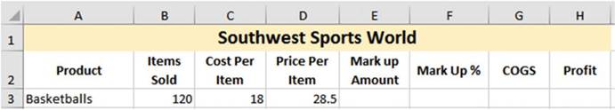
Figure7-5.Enterthisdatainyourownworkbook
Table 7.3 shows the formulas needed for each unfilled column.
Table7-3.FormulasNeededforSpreadsheet

Spreadsheet
Formulas
Markup Amount� Price Per Item � Cost Per Item Markup %��� Cost Per Item / Price Per Item
COGS����� Items Sold
* Cost Per
Item
Profit����� (Items Sold * Price
Per Item) - COGS
Computing
the Markup Amount
1.
Enter an equal sign (=) in cell E3. Enter d. Excel knows you are entering
formulas and so it tries to be helpful by suggesting one of Excel�s
built-in functions that starts with a D. See Figure 7-6.
223
CHAPTER 7 ■ CREATING AND USING
FORMULAS
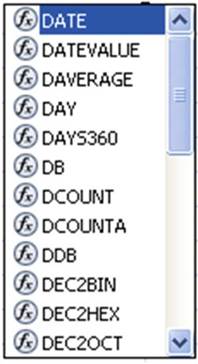
Figure 7-6. Built-in functions
2.
We will look at built-in
functions later, but for now ignore the function choices
and just enter
d3. Excel provides a visual cue for your selection by putting a box around
the cell that you entered
in your formula.
It makes the cell address
and the box both blue. See Figure
7-7.
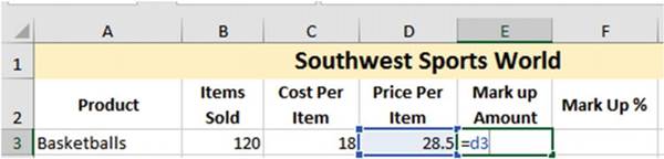
Figure 7-7.Cell
address and its corresponding cell are the same color
3.
Enter a minus sign (-) then c3. Excel makes
the cell address
and the box surrounding the referenced cell both red. See Figure
7-8.
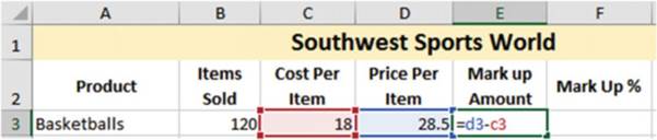
Figure 7-8.Cell
address and its corresponding cell are both red
224
CHAPTER 7 ■ CREATING AND USING
FORMULAS
4.
Press Ctrl + Enter. The cell displays
the value returned
from the formula.
The formula bar, however, shows the formula
entered in the cell. See Figure 7-9.
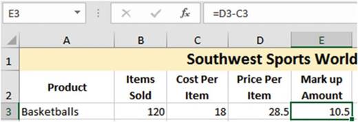
Figure7-9.Formulabardisplaystheformulaenteredintheactivecell
Computing
the Markup %
1.
Enter an equal sign (=) in cell F3. This time instead of entering cell addresses in the
formula,
you will click the cell you want to use and Excel will automatically put the address
of that cell in your formula. Click
cell C3. Excel places
an animated box around cell C3 and places its address in the formula.
2.
Enter a divide sign (/).
3.
Click cell D3. See Figure 7-10.
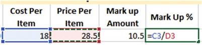
Figure 7-10. Formula entered for Markup %
4.
Press Ctrl + Enter. The result is 0.631578947. This number might be rounded depending
upon the width of the column.
5.
We would like to show the value as a percentage. Select
the Home tab if it isn�t
already selected then click the % icon in the Number group.
The result is rounded up to 63%.
6.
We would like to have the number displayed with two decimal
positions. Click the increase decimal button
 �twice. The
value changes to 63.16%.
�twice. The
value changes to 63.16%.
Computing
the Cost of Goods Sold
1.
Click cell G3 and enter =b3*.
2.
Click cell C3 and press the Tab key.
225
CHAPTER 7 ■ CREATING AND USING
FORMULAS
Compute
the Profit
1.
Click inside cell H3. You can
use any combination of typing the cell reference or clicking the cell to get its reference for the profit
formula. Enter the formula
=(b3*d3)�g3 in
cell H3.
2.
Press Enter. See Figure 7-11.
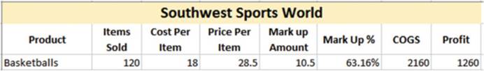
Figure7-11.Resultofenteringformulaforprofit
Copying
Formulas
You used the Fill Handle previously to AutoFill a series of values. The Fill Handle can also be used to copy
formulas across rows or columns while it automatically adjusts the formula for the proper column and row.
If you copy formulas down through a column, the row number in the formula will be automatically adjusted to
the current row where the formula is being copied to. If you copy formulas across rows, the column letter in
the formula will be automatically adjusted to the current column of where the formula is
being copied to. This automatic adjustment of row and column addressing is called relative cell
referencingbecause the cell addresses change relative to where the formula is placed.
This exercise continues with the same worksheet from the previous
exercise. You will add additional records and then copy the formulas you made previously into the new rows.
1.
Add the additional records (rows 4�7) shown in Figure 7-12.
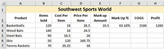
Figure7-12.Addtheseadditionalrecords
226
CHAPTER 7 ■ CREATING AND USING
FORMULAS
2.
Click in cell E3. Drag the AutoFill
Handle down from cell E3 through cell E7. See Figure 7-13.
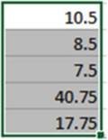
Figure 7-13.Result
of dragging the AutoFill Handle
down from cell E3 to cell E7
AutoFill copies the formulas to the other cells automatically. When AutoFill is used to copy formulas
down through a column it automatically adjusts
the cell references in the formula
to the current row.
3.
Click cell E4. The formula in
cell E4 is =D4-C4. The row was adjusted from 3 to
4.
4.
Click other cells in the column to see how their formulas were adjusted.
5.
Drag the AutoFill Handle down
from cell F3 through F7.
6.
Drag the AutoFill Handle down
from G3 to G7.
7.
Drag the AutoFill Handle down from H3 to H7. Your result
should look like Figure 7-14.
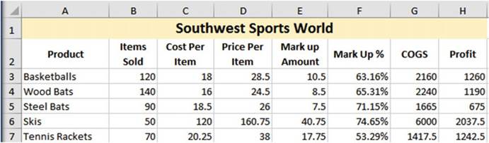
Figure7-14.Resultofcopyingformulas
227
CHAPTER 7 ■ CREATING AND USING
FORMULAS
You have seen how the AutoFill
Handle automatically adjust the row reference
when copying formulas
down in a column. Now we will look at how the AutoFill Handle
can be used to automatically adjust the column reference when copying formulas
across a row.
1.
Create a new worksheet named �ColumnRef.� Enter the values
as shown in cells A1:D2.
A colon between
two cell addresses means the range between the cells. The first cell address, in this case A1, is the
upper-left-hand cell of the range. The second cell address, in this case D2, is the bottom
right cell of the range.
See Figure 7-15.
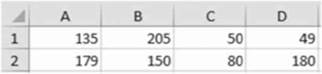
Figure7-15.Enterthesevalues
2.
Enter = a1-a2 in cell A3. See Figure
7-16.
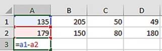
Figure 7-16. Enter formula in cell A3
3.
Press Ctrl + Enter.
4.
Drag the AutoFill Handle in
cell A3 across through cell D3.
Figure 7-17 shows
the result of using the AutoFill
Handle to copy the formula from cell A3
to cells B3, C3, and D3.
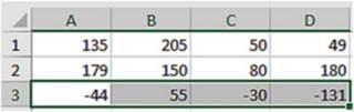
Figure7-17.Resultofusingcopyingformula
You can see in Figure 7-18 that Excel adjusted the column in the cell reference when it copied the formula
228
CHAPTER 7 ■ CREATING AND USING
FORMULAS
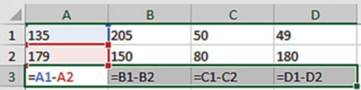
Figure
7-18. Copied formula
You�ve learned how to enter formulas. Next, you will use Excel�s AutoCalculate Tools. These tools allow you
to select a range of data and then click the Calculate tool you need. The formula is automatically
applied to that data without you having to enter it.
AutoCalculate Tools
The AutoCalculate Tools
feature includes tools for summing, averaging, counting the number of cells
that contain numeric data, and finding the largest or smallest value in a cell
range.
AutoSum
The AutoSum feature
provides a quick way to sum a range of numbers. The range could consist of a
single cell or thousands of cells. The AutoSum feature automatically adds values
that are in a contiguous range.
A contiguous range
is one in which there
are no empty cells.
The AutoSum
feature is located on the Ribbon�s Home tab in the Editing group. The icon for
the AutoSum feature is the Greek capital letter Sigma
 . Math and Science use
 �as a summation operator. See Figure 7-19.
Figure 7-19. AutoSum feature
When you click the AutoSum button,
Excel first checks
to see if there are any values
above the current cell. If there are, Excel will sum the values above
it; otherwise, it will check
to see if there are values to the left of it and if there
are it will sum those
values.
In Figure 7-20 cell F2 was selected when the AutoSum
button was pressed. Excel highlighted the numeric values to its left. If only
one cell is selected when you click the AutoSum button the Sum formula will display with the range of values
that is being summed. If this isn't the range you want to sum, then you can change either the starting or
ending cell addresses.
229
CHAPTER 7 ■ CREATING AND USING
FORMULAS
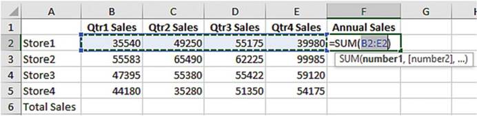
Figure 7-20.Excel selects numeric
values to the left when using AutoSum
and displays the range that it is going to use
Clicking the
AutoSum button a second time or pressing the Enter key will display the results
as shown in Figure 7-21. The formula bar is displaying the
formula created by AutoSum.
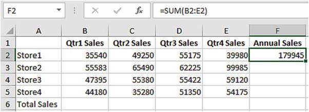
Figure 7-21.Clicking AutoSum a second time enters the resulting
value in the cell
Figure 7-22 shows the results of having used the AutoFill Handle to copy the formula down through cell F5.
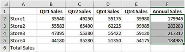
Figure7-22.Resultsofcopyingformula
230
CHAPTER 7 ■ CREATING AND USING
FORMULAS
Since we are summing rows, Excel automatically adjusted the row address for each of the copied cells.
�
Cell F3 contains the formula =SUM(B3:E3).
�
Cell F4 contains the formula =SUM(B4:E4).
�
Cell F5 contains the formula =SUM(B5:E5).
Next, we will look at adding both the columns and the rows at the same time, but before we do that let�s
look at how you would clear the totals from column F.
The
cell contents can be cleared
by first selecting the cells to clear and then doing
one of the following:
�
Clicking the Clear
button
 �in the Editing
Group and then selecting Clear Contents
�in the Editing
Group and then selecting Clear Contents
�
Right-clicking the selected range
and then selecting Clear Contents from the context
menu
Totaling the columns and rows all at once is done by first selecting the
row and column cells where the totaled results will be placed. In the spreadsheet in Figure 7-23, you would
do it by selecting cells
F2:F5 and then holding down the Ctrl
key and selecting cells B6:F6.
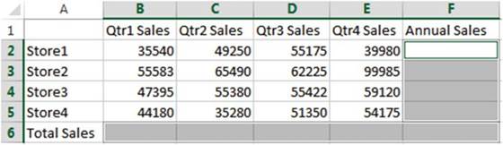
Figure 7-23.Holding down the Ctrl key lets you select
mutliple cell ranges
Clicking the AutoSum button now will sum both the rows and columns. See Figure 7-24.
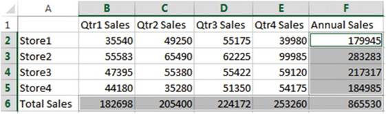
Figure7-24.Resultofsummingrowsandcolumns
A faster way of summing the rows and columns for a range of values is to select the values themselves
along with one column to the right and one row below as shown in Figure 7-25.
Then press the AutoSum button. The result will be the same as Figure 7-24.
231
CHAPTER 7 ■ CREATING AND USING
FORMULAS
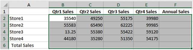
Figure 7-25.Select
data plus the column to right and one row below before
clicking AutoSum
Handling Blank Cells
in a Range
AutoSum does not include any cells in its range after reaching a blank cell. See Figure 7-26. : If you wanted
to include cell A2 in the total you would need to change A4 in the formula to cell A2.
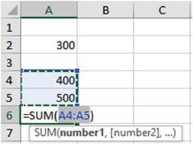
Figure7-26.ChangeA4intheSumfunctiontoA2
Another way to
change the range is to take one of the handles of the selected range and drag
it so that it includes all the cells you want, as shown in Figure 7-27.
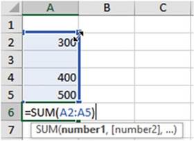
Figure7-27.Dragselectionhandletoincludecellsyouwantincluded
232
Average, Count Numbers,
Max, Min
CHAPTER 7 ■ CREATING AND USING
FORMULAS
If you click the down arrow besides the AutoSum button (Figure 7-28) you can see that Excel includes several
other �Auto� functions. The functions are Average, Count Numbers, Max(imum), Min(imum), and More Functions.
These �Auto� functions work the same way as AutoSum.
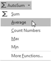
Figure 7-28. Auto functions
In this exercise
you will apply the AutoCalculate Tools AutoSum, Average,
Max, and Min across rows and columns.
1.
Create a new worksheet named �AutoCalculate.�
2.
Select cells B1:I1, which will be the cells containing your column headings. On the Home tab in
the Alignment group click the Wrap Text button. See Figure 7-29. Now your column
headings will wrap and not be partially
hidden.
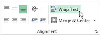
Figure 7-29. Select Wrap Text
3.
Enter the data for the workbook as shown in Figure 7-30.
233
CHAPTER 7 ■ CREATING AND USING
FORMULAS
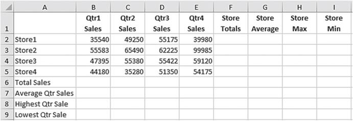
Figure 7-30. Enter this data
4.
Select the cell range B6:E6. Click
the AutoSum button.
5.
Select the cell range B2:E5.
Click the down arrow next to the AutoSum button.
Select Average.
■
Note� When you use an �Auto�
function Excel will place the results in the first blank row below the selected range when the range is in a
column or, as in our case, include both rows and columns. If the range is just in a row, Excel
places the result to the right of the range.
6.
Cell range B2:E6
is currently
selected. Change the selection
back to
B2:E5. Click the down arrow next
to the
AutoSum button. Select Max. The
Max function
returns the highest value in
a selected
column or row. Store 2 sold
the most
in each
quarter.
7.
Select the cell range B2:E5 again. Click
the down arrow next to the AutoSum
button. Select Min. See Figure 7-31. The Min function returns
the lowest value in a selected column
or row. Store1 sold the least in quarters 1 and 4. Store4 sold the least in quarters
2 and 3.
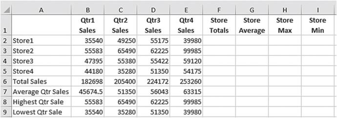
Figure7-31.ResultofusingAutoFunctions
234
CHAPTER 7 ■ CREATING AND USING
FORMULAS
8.
Select cells F2:F5. Click on the AutoSum button.
9.
Select cells B2:E2. Click on the down arrow of the AutoSum
button. Select Average.
Click cell G2. Use the AutoFill Handle
to drag the formula down through cell G5.
10.
Select cells B2:E2. Click the down arrow of the AutoSum button.
Select Max. Click cell H2. Use the AutoFill Handle
to drag the formula down through cell H5.
Let�s look at another
way of doing this.
1.
Click cell I2. Click
the down arrow of the AutoSum
button. Select Min. See Figure 7-32. The function displays and a
marquee appears around cells B2:H2. This
is not the range we want.
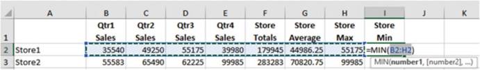
Figure 7-32. Wrong range selected
2.
Select cells B2:E2. The formula
will adjust accordingly. See Figure 7-33.
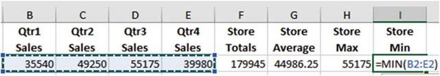
Figure7-33.UsetherangeB2:E2forthefortheMINfunction
3.
Press Ctrl + Enter. Use the AutoFill
Handle to copy the formula
down through cell I5. See Figure 7-34.
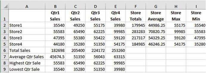
Figure7-34.UseAutoFillHandletocopytheformuladownfromI2toI5
235
CHAPTER 7 ■ CREATING AND USING
FORMULAS
4.
Let�s improve the look of the spreadsheet. Let�s add commas to make it easier to read and color to
distinguish the original data from the computed data.
5.
Type A1:I9 in the Name Box then
press Enter.
6.
On the Home tab in the Styles
group click the Cell Styles
More button. See Figure 7-35. Figure
7-36 shows what appears after
clicking the Cell Styles More button.
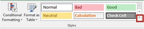
Figure7-35.ClicktheMorebuttontoviewmorestyles
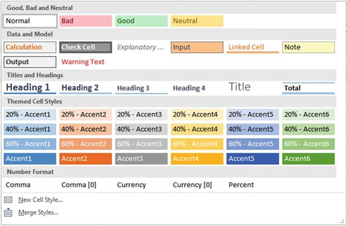
Figure 7-36. All of the Cell Styles
7.
Move your cursor
over Comma[0] in the Number Format area. You can see how selecting this option will affect your worksheet by
changing the data to having commas
with no decimal position. Click
Comma[0].
8.
Enter A1:E5 in the Name Box then
press Enter.
9.
On the Home tab in the Styles group click the Cell Styles More button.
236
CHAPTER 7 ■ CREATING AND USING
FORMULAS
10.
In the Data and Model area click Input.
11.
Use the border
button in the Font group
to create a thick outside
border around the same cells.
See Figure 7-37.
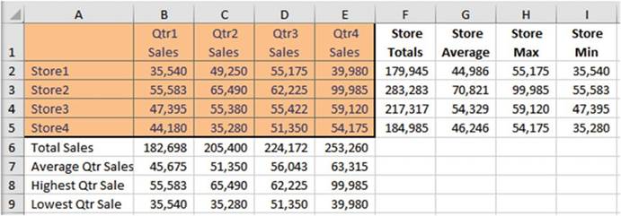
Figure 7-37. Thick outside border
You�ve learned
how to enter formulas manually and by using Excel�s AutoCalculate tools. When
viewing the worksheet, you see the
results of formulas but not the formulas themselves. In order to see the
formula, you need to click the cell that contains the formula and then view it in
the formula bar.
Viewing Formulas
Clicking a cell that contains a formula will display the formula in the formula bar, but wouldn�t it be nice
to see all of your formulas at once? You can do this by holding down the Ctrl key and pressing the
Tilde Key (~).
You can print your spreadsheet while all of the formulas are visible. This gives you a record of your
formulas and provides a convenient way of overviewing your work to make sure all of your formulas have been
entered correctly. Figure 7-38 shows the results of using Ctrl + ~.
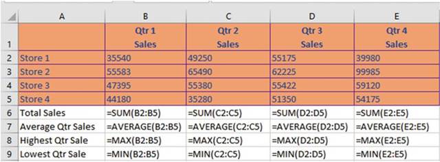
Figure 7-38. Formula view
You can return to normal view by clicking Ctrl+~again.
237
CHAPTER 7 ■ CREATING AND USING
FORMULAS
Creating Named Ranges and Constants
Up to this point we have
been using cell addresses in our formulas, but when we are thinking about computations we don�t normally
think
of cell addresses; we usually think in descriptive words. For example, when computing the company payroll, I
am thinking Hours*Ratenot B2*C2. We can also assign names to
values that we know will not change.
For example, I can assign the name PI a value of 3.14 and then use the word PIin
my formulas rather than the value 3.14.
Naming Ranges
We can assign a descriptive
name to a range of cells and then use that name in our formulas. A name is assigned to
a range of cells by selecting those cells and then entering a name for that
range in the NameBox. See Figure 7-39.
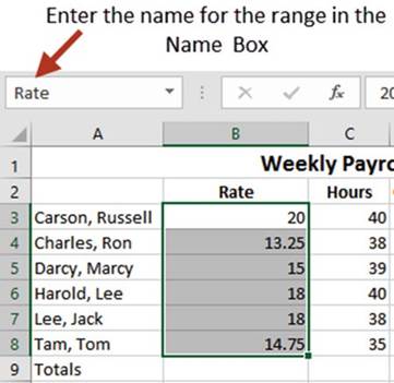
Figure7-39.EnterrangenameintheNameBox
Names can�t be
longer than 255 characters and they must start with a letter, underscore, or
backslash. Names are not case sensitive. Clicking the down
arrow next to the Name Box displays a list of all the named ranges in
the workbook. Clicking one of them will highlight the cells belonging to that
named range.
■
Note� A common mistake people make is that they do not press the Enter key after
they have entered a name in the Name Box. If you do not press the Enter key, the name will not be saved.
Another way of creating named ranges is to use the options available in the Defined Names group which is
located on the Ribbon�s Formulas tab. See Figure 7-40.
238
CHAPTER 7 ■ CREATING AND USING
FORMULAS
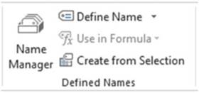
Figure 7-40. Defined Names group
Clicking the Define Name button brings up the NewName dialog box. See Figure 7-41. You can
either select the cells you want to become a named range before you open the New Name dialog box or wait
until it is opened and then select a range. You can also bring up the New Name dialog box by right-clicking
the spreadsheet and selecting DefineName from the context menu. Creating a named range by
using the New Name dialog box gives you a couple of options that would not be available if you just entered
a name in the Name Box.
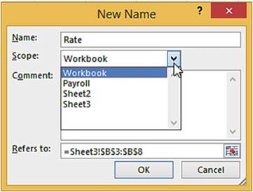
Figure 7-41. New Name dialog
box
The Name textbox in the New Name dialog box uses the column or row heading by default for the cells
you
selected before opening
the New Name dialog box. You can change the name to whatever you want.
The purpose
of the Scope drop-down box is to let you select whether
you want to make the named range
available for formulas
in the entire workbook or for just a particular worksheet.
You can enter a Comment. The comment does not appear on the worksheet. It will appear only in the
Name Manager which we will look at shortly. You can also name ranges in the Name Manager.
The Refers to text
box displays the range address
of the selected cells. If you haven�t
already selected the cells you want to name before
you bring up the New Name dialog
box you can select them at this time.
Naming Noncontiguous Ranges
To create a named range for
a group of noncontiguous cells, select the cells while holding down the Ctrl� key and then enter a name for
the group. In Figure 7-42 you could assign an appropriate name
for all of the
Quarter 1
values such as QTR1. You could add all of the Quarter 1 values by entering =SUM(QTR1) in a cell or find the
average value by entering =AVERAGE(QTR1).
239
CHAPTER 7 ■ CREATING AND USING
FORMULAS
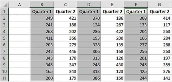
Figure7-42.Createanamedrangefornoncontiguouscells
Naming Constants
You can also use the New Name dialog box to assign names to constants. A constant is a value that doesn�t
change. For example, you can assign names to interest or tax rates. Enter the name you wish to assign to the
constant in the Nametext box. Next, replace
the current cell address in the Refers to text
box with the constant value. If you are entering
a constant that is a percent, you can enter the value with a percent sign such
as 4.5%, or you could enter the decimal equivalent of .045. See Figure 7-43. Assigning a name to a constant
lessens the chance of errors.
If I used the tax rate of 4.5% in ten cells and now the tax rate changes
to 4.7%, how many cells am I going to
have to change? That�s right I would have to find the ten cells and then change all
of them. But, if I used a constant I would just change the constant value once
to 4.7%.
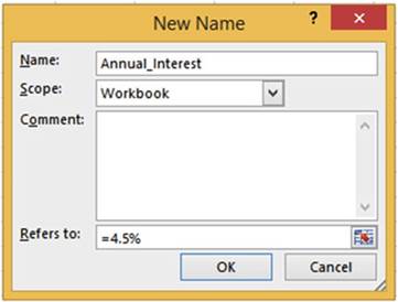
Figure7-43.Assignanametoaconstant
240
Name Manager
CHAPTER 7 ■ CREATING AND USING
FORMULAS
Clicking the Name Manager button in the Defined Names group displays the Name Manager which lists the named
ranges and constants. The Name Manager has buttons for Adding, Editing, and Deleting named ranges. It also
has a Filter option for limiting which named ranges to display.
You can see in Figure 7-44 that the named range Rate had values in its range when it was created. The
Gross Pay and Hours ranges were created before any values were placed in their cells.
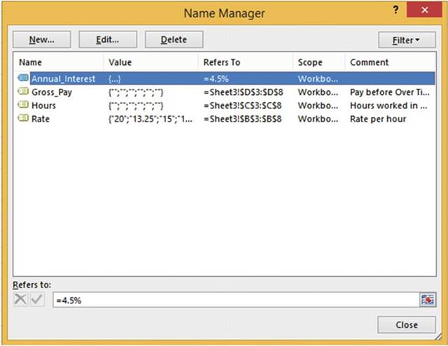
Figure
7-44.RangenameRatehasvaluesinitbecausetheyweretherewhentherangewasselected
Editing Named Ranges and Constants
Clicking the Newbutton in the Name Manager window brings up the same New Namedialog box we saw
when we clicked on the Define Name button in the Defined Names group. To edit a named range select the range
you wish to edit from the list and then click the Editbutton. The Edit Name dialog box (Figure 7-45)
is similar to the New Name dialog box. From here you can change the Name, the Comment, and the location of a
range or change the Constant value.
241
CHAPTER 7 ■ CREATING AND USING
FORMULAS
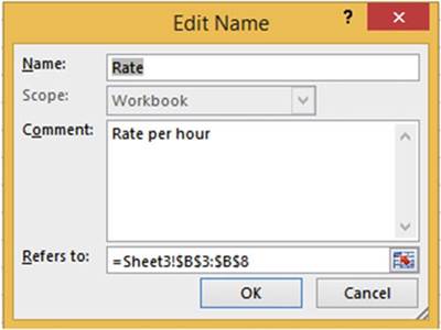
Figure 7-45. Edit Name dialog
box
Deleting Named Ranges and Constants
The only way to remove a
named range is to use the Name Manager. First you select the range(s) you want
to remove and then press the
Delete button. This brings up a warning dialog box that asks you to confirm the deletion (Figure 7-46).
Removing a named range only removes
the name associated with a range of cells. It does not remove the cells or the data
in them.
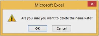
Figure 7-46.Message confirming that you want to
delete the named range
Using Column or Row Headings
for Range Names
If you are
going to create named ranges for multiple rows or columns, you may find it
easier to let Excel use your
row or column headings as names for the named ranges. To do this you would
first select the cells that your named ranges would include along with their
column or row headings. See Figure 7-47.
242
CHAPTER 7 ■ CREATING AND USING
FORMULAS
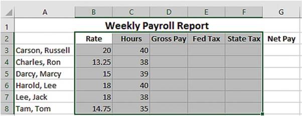
Figure 7-47.Select
headings along with data when creating range names for multiple rows or columns
You would then click the Create from Selection button in the Defined
Names group. See Figure 7-48.
This would bring up the Create Names from Selection dialog box (Figure 7-49).
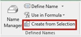
Figure7-48.CreatefromSelectionbutton
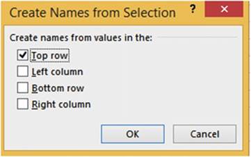
Figure7-49.CreateNamesfromSelectiondialogbox
You would
need to select
Top row to get the column headings. Excel would assign
the named ranges
as follows:
�
Rate to cells
B3:B8
�
Hours to cells
C3:C8
�
Gross_Pay to cells D3:D8
243
CHAPTER 7 ■ CREATING AND USING
FORMULAS
�
Fed_Taxto cells E3:E8
�
State_Tax to cells F3:F8
■
Note� Named ranges can�t contain spaces.
Excel puts an underscore in place of spaces when it uses row
or column headings.
Selecting Named Ranges
Rather Than Typing
Them into Formulas
You can type named
ranges directly into a formula
such as =Rate*Hours. If you don�t
remember the name assigned to a range
or you want to be sure you don�t misspell
it, you can use the Use in Formula
button in the Defined
Names group. See Figure 7-50.
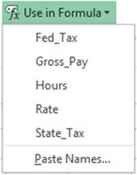
Figure 7-50. Use in Formula
button
If you are just
starting a formula, clicking one of the named ranges will place the equal sign
along with the named range in the
formula. For example, using our payroll example, we want to compute the gross
pay in cell D3 by multiplying
Rate times Hours. You would click inside cell D3 and then click the Rate in the
UseinFormulalist box. This would create
=Rate. You would then type the *
for multiplication. You would finish the formula by clicking Hours and then pressing the Enter key.
A quicker way to select named ranges or constants is to press F3. Pressing F3 brings up all the available
names for you to select from.
244
CHAPTER 7 ■ CREATING AND USING
FORMULAS
In this exercise you will create range names
using different methods. You will
also create constants that will hold the tax values.
1.
Type the data into a new worksheet as shown in Figure 7-51.
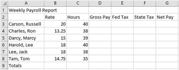
Figure 7-51. Enter data
2.
Format the title:
a.
Select cells A1:G1.
b.
Click the Merge & Center button located on the Home tab in the Alignment group.
c.
Bold the text.
d.
On the Home tab, in the Font
Group, click the Increase Font Size button twice.
3.
Center and bold the column
headings. Your spreadsheet should
now look like Figure 7-52.
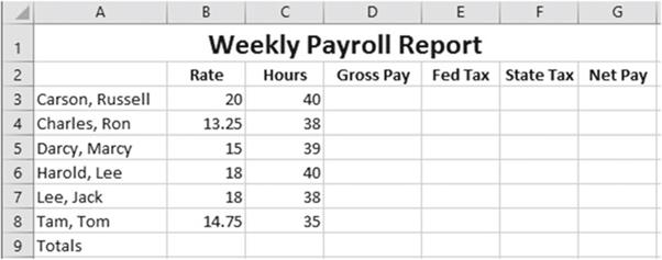
Figure7-52.Formattedworksheet
245
CHAPTER 7 ■ CREATING AND USING
FORMULAS
Creating
Named Ranges Using the Name Box
1.
Select cells B3:B8.
Type Rate into the Name Box. Press Enter.
2.
Select cells C3:C8. Type Hours into
the Name Box. Press Enter.
3.
Select cells D3:D8. Type GrossPay into
the Name Box. Press Enter.
4.
Select cells E3:E8. Type FedTax into
the Name Box. Press Enter
Creating
Named Ranges Using Define Name
1.
Select cells F3:F5.
2.
Right-click any one of the selected
cells. Select Define Name from the context menu. Excel assigns a name of
State_Tax to the range. Excel got the name from the column heading. Names can�t contain
spaces; therefore Excel filled in the space with an underscore. The Refers to text box contains the
selected range.
3.
Click the OK button.
Changing
a Name or Its Range
You
can�t change
a name
or its
range in
the Name
Box. These
changes can only be done
through the Name Manager. The
State
Tax range is currently F3:F5
but it
needs to
be changed
to F3:F8. Let�s
also change
the name
by removing
the underscore.
1.
On the Formulas tab in the Defined Names group click the Name Manager
button.
2.
Click State_Tax. Click
the Edit button.
The Edit Name dialog box appears.
3.
Remove the underscore from the name so that the name is StateTax.
4.
Tab to the Refers to text
box. See Figure
7-53. An animated
marquee appears around
cells F3:F5.
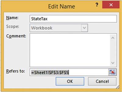
Figure7-53.Changetherangenameandlocation
246
CHAPTER 7 ■ CREATING AND USING
FORMULAS
5.
If you can�t see cells F3:F8, then
move the Edit Name window over until you can.
6.
Drag across the cell range
F3:F8. Click the OK button. Click the Close button.
7.
Click the down arrow of the Name Box. It should display all of your named
ranges. See Figure 7-54.
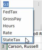
Figure7-54.RangenamesdisplayedinNameBox
8.
Click StateTax. This highlights
the StateTax range.
9.
Select the cell range B3:B8
on the worksheet. The name box should
now display the name Rate.
Changing
the Size of the Name Box
1.
Since your names
can be as long as 255 characters you might need to widen
the Name Box to see more of the name.
2.
Move your cursor to the right of the Name Box. When the cursor changes to a
horizontal double arrow drag to the right to increase the size of the Name Box. As you increase the size of
the Name Box, the function area shrinks and vice versa.
Drag to the left to decrease the size of the Name Box. See Figure 7-55.

Figure7-55.ChangethesizeoftheNamebox
Removing a
Named Range
1.
Click the Formulas tab
on the ribbon.
2.
In the Defined Names group click the Name Manager
button. The Name Manager displays
the existing named
ranges. They are displayed in alphabetic order.
3.
To select all of the named ranges
click FedTax then hold down your Shift
key and click
StateTax.
4.
Click the Delete button in the Name Manager window.
247
CHAPTER 7 ■ CREATING AND USING
FORMULAS
5.
A dialog box appears asking �Are
you sure you want to delete the selected names?�
6.
Click the OK button.
7.
Click the Close button.
Creating
Named Ranges Using Create from Selection
1.
Select cells B2:F8
2.
In the Defined Names group click the Create
from Selection button
3.
Select Top Row from
the Create Names from Selection dialog box. Click the OK
button.
4.
Click the Name Manager button.
The named ranges were created
from the column
heads. Spaces in the column names were replaced with an underscore. See Figure 7-56.
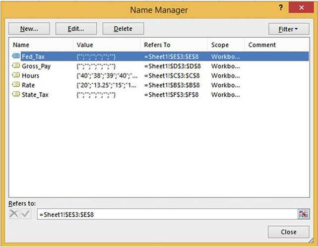
Figure7-56.Rangenamescreatedfromcolumnheads
5.
Click the close button.
248
CHAPTER 7 ■ CREATING AND USING
FORMULAS
Creating
Named Constants
For the
purposes of this example let�s just say the federal tax is 32%. We will assign a named constant to this
value.
1.
In the Defined Names group click the Define
Name button.
2.
Type FederalTaxRate in the Name
text box.
3.
Type Fictitious Federal Tax rate
for practice example in the Comment box.
4.
Type =32% in the
Refers to text box over the existing text. See
Figure 7-57. If you prefer you can use the decimal equivalent
and type =.32.
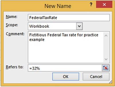
Figure 7-57.Name
of FederalTaxRate assigned
to the constant 32%
5.
Click the OK button. Let�s say the state tax is 8%.
1.
Click the Define Name button.
2.
Type StateTaxRate in the Name text box.
3.
Type Fictitious State Tax rate
for practice example in the Comment box.
4.
This time let�s use the decimal equivalent of 8%. Type =.08
in the Refers to text box. See
Figure 7-58.
249
CHAPTER 7 ■ CREATING AND USING
FORMULAS
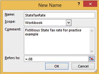
Figure 7-58.Name
of StateTaxRate assigned
to the constant .08
5.
Click the OK button.
6.
Click the Name Manager button.
You can see that the new constants
have been added.
7.
Click the Close button.
8.
Click the down arrow for the Name Box. As you can see, constants do not appear
in the Name Box. This is because
they don�t refer
to any particular cell.
Using
Named Ranges in Formulas
1.
In cell D3, enter
=R.
Excel brings up a list of all the built-in functions that start with R
as well as all named ranges that start with R.
See Figure 7-59.
250
CHAPTER 7 ■ CREATING AND USING
FORMULAS
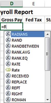
Figure7-59.Built-infunctionsandnamedrangesthatstartwithR
Named ranges are easily distinguishable from functions because
they have a different icon in front
of them. The
 �icon represents named
ranges. Notice that there is a Rate named range which you created and a RATE function. We want
to use the Rate with the
�icon represents named
ranges. Notice that there is a Rate named range which you created and a RATE function. We want
to use the Rate with the
 �icon in front of it.
2.
Click the
 Rate and then press the Tab key. After
pressing the Tab key Excel places a rectangle around
the cells that are a part of the named range. See Figure 7-60.
Rate and then press the Tab key. After
pressing the Tab key Excel places a rectangle around
the cells that are a part of the named range. See Figure 7-60.
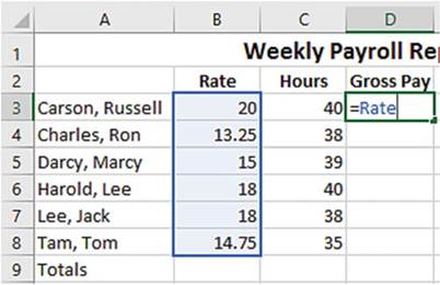
Figure 7-60.When
entering a range name Excel highlights the cells in that range
251
CHAPTER 7 ■ CREATING AND USING
FORMULAS
3.
Type *Ho. See Figure
7-61.
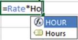
Figure 7-61.Typing
Ho brings up the intellisense choices for the function Hour and the named range Hours
4.
Use the down arrow to select
 �and then press the Tab key. Excel places
a different color rectangle around
the cells that encompass the Hours range.
�and then press the Tab key. Excel places
a different color rectangle around
the cells that encompass the Hours range.
5.
Press Ctrl + Enter.
6.
Use AutoFill to copy the formula down through cell D8.
7.
Click cell D4. Look in the formula
bar. The formula
for every cell in the column will show
=Rate*Hours. You won�t see any row adjusting as you do when you are using cell references in your
formulas.
Selecting
Named Ranges from Use in Formula
1.
Click inside cell E3. On the Formulas
tab in the Defined Names group click the Use in Formula button. Select FederalTaxRate
2.
Type * (asterisk).
3.
Click the Use in Formula button. Select Gross_Pay.
4.
Press Ctrl + Enter.
5.
Use the AutoFill Handle to copy
the formula down through cell E8.
6.
Click inside cell F3. On the Formulas
tab in the Defined Names
group click the Use in Formula
button. Select StateTaxRate
7.
Type * (asterisk).
8.
Click the Use in Formula button. Select Gross_Pay.
9.
Press Ctrl + Enter.
10.
Use the AutoFill Handle to copy
the formula down through cell F8.
Setting
the Scope for a Name
The scope of a name is where that name can be used. The scope can pertain to an entire
workbook or to an individual worksheet. When you create a named range
using the Name Box, the named range
has a scope of the entire workbook. In other words,
you can use that named
range on any worksheet in the workbook
that you declared
it in. It doesn�t matter
how many worksheets are in the workbook; it will work on any of them.
Let�s see what happens when we declare
a scope of an individual worksheet for a named range
or named constant.
252
CHAPTER 7 ■ CREATING AND USING
FORMULAS
1.
Add another worksheet to the workbook. Change the name on the worksheet tab to
�TestScope.�
2.
Select the cell range A1:A5.
3.
On the Formulas
tab on the Ribbon in the Defined
Names group click the Define Name button.
4.
Type SheetScopefor the Name.
5.
Click the down arrow for Scope and select TestScope. The Refers to text box should reflect
that you have selected the range A1:A5.
See Figure 7-62.
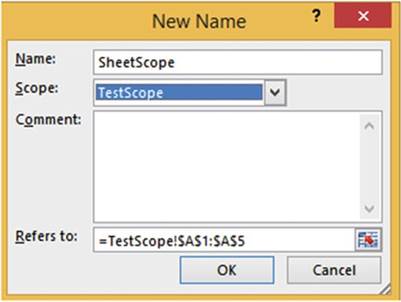
Figure7-62.RangeA1:A5isselected
6.
Click the OK button.
7.
Press F3. The SheetScope range appears in the
list along with the Names you created previously. Since the other names were created
with a scope of
Workbook
they are accessible from any worksheet.
8.
Click the Cancel button.
9.
Click another worksheet. Press F3. SheetScope will not appear
in this list because its scope is limited to the TestScope worksheet.
10.
Click the Cancel button.
11.
Click the Name Manager button. Click the Filter button. Select Names Scoped to Worksheet.
See Figure 7-63. SheetScope is the only
Name displayed because it is the only one whose scope is limited to a
worksheet.
253
CHAPTER 7 ■ CREATING AND USING
FORMULAS
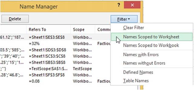
Figure7-63.SelectNamesScopedtoWorksheet
12.
Click the Filter
button again. Select Names Scoped
to Workbook. All the Names are displayed
except for SheetScope.
■
Note� If you assign a name with a scope of worksheet you can create a range on
another worksheet with that same name.
13.
Click the Close button.
Now you�ve seen
how to simplify formulas by using named ranges and constants. Up to this point, when you
copied a formula down a column or across a row, the formula automatically
adjusted for the row or column change, but there are times when you don�t
want that to happen. You learn how to prevent these changes in
the next section.
Absolute Cell References
As you have seen when using
relative cell addressing with the AutoFill
feature the cell addresses are adjusted automatically. As you will see relative cell referencing
doesn�t work for every situation.
Binder Corporation is thinking about
giving each of its employees
a 5% raise. Each employee�s salary is listed in column B under the heading Current
Salary. The amount
of the increase for each employee is to be displayed in column C. The formula
in column C4 is entered
as =B4*B1. See Figure
7-64. The result is 2087.5. This is the result
of taking 41750
* 5%.
254
CHAPTER 7 ■ CREATING AND USING
FORMULAS
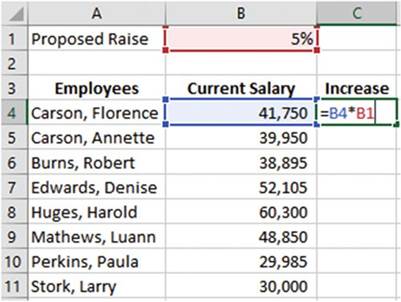
Figure7-64.Theformulafor5%raiseisenteredincellC4
Say you use the AutoFill Handle to copy the formula for the rest of the employees. Figure 7-65 shows the
resulting copied formulas.
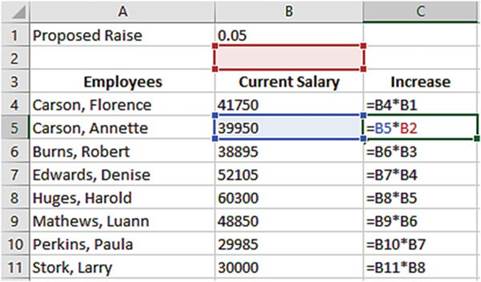
Figure7-65.FormulasafterbeingcopiedwithAutoFillHandle
Looking at our
formulas we can see that we are headed for trouble starting with cell C5 and
continuing down through the other
formulas. The row portion of the relative
cell address B1 was automatically adjusted from 1 to 2. Since there is no value
in B2, the value 39950 will be multiplied by 0 giving the result of 0.
Figure 7-66 shows the results
of the formulas.
255
CHAPTER 7 ■ CREATING AND USING
FORMULAS
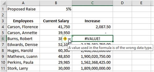
Figure7-66.Resultsofformulanotwhatwewanted
Figure 7-65 shows that the formula
in cell C6 is =B6*B3. Cell B3 contains
the alphabetic data �Current Salary.� You can�t use alphabetic data in a formula, which is why it shows the
error #VALUE!. If you click the smart tag next to the error Excel displays
a tool tip which states that the value used in the formula is of the wrong data type.
Cell C7
multiplies 52105 * 41750. This is clearly not what we want. We do not want
Excel to perform any automatic adjusting for cell B1.
If you want
formulas to refer to a single cell you need to use absolutecellreferencing. Absolute
cell referencing locks the cell address in a formula so that when you copy it,
it doesn�t automatically adjust� for the row or column
change. Absolute cell addresses are made by placing a dollar sign in front of
both the column and the row.
This can be done by manually typing them in or you can type the address as you normally do then press F4.
Pressing F4
places a $ sign in front of both the column and the row.
In our example if we entered
the formula =B4*$B$1 in cell C4 then used the AutoFill handle
to copy the formula down through cell C1, the formulas would
look like those in Figure
7-67.
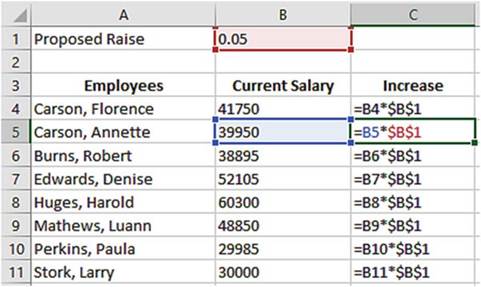
Figure 7-67.Making cell B1 an absolute address in
the formulas in column C
256
CHAPTER 7 ■ CREATING AND USING
FORMULAS
The
result would be as shown in Figure
7-68. This is what we wanted.
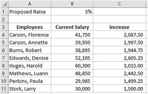
Figure7-68.Resultofusingabsolutecellreferencing
In this example
you will create a travel expense report for the second quarter
of 2015. You will add computations for computing the mileage expense
and the total amount of travel expenses
for the quarter. You will then compare
the quarter totals to the same quarter
in 2014 and determine the dollar amount
and percent difference between the two.
1.
Create a new worksheet named �Absolute.� Make your
worksheet look exactly like the one in Figure 7-69.
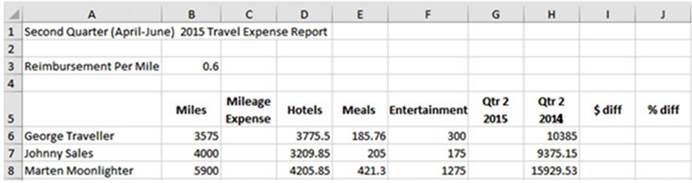
Figure 7-69.Enter
the data here in a new worksheet
named Absolute
2.
Merge and center the title in row 1 across cells A1: J1. Click the Increase Font Size button
twice.
3.
Center the column headings both vertically and
horizontally. Bold the column
headings.
257
CHAPTER 7 ■ CREATING AND USING
FORMULAS
4.
Compute the values for the Mileage Expense
column by taking the miles traveled times the reimbursement rate per mile. The reimbursement rate stored in
cell B3 is 60 cents for every mile traveled.
a.
In cell C6 enter the formula =B6*B3.
b.
Use the AutoFill handle and
drag the formula down through C8.
Problem:
Cell C8 displays
#Value!. Click cell C8. Look at the formula in the formula
bar. The formula
is =B8*B5. The formula
adjusted for the row when you used the AutoFill
handle. Cell B5 contains the text �Miles.�
If you use text in a formula
Excel displays a #Value error.
Fix the Problem:
Since you
want to use cell B3 in each formula you will need to make it absolute.
5.
Move your cursor in front of B3 in the formula in Cell C6
then press F4 to make the cell address absolute. Your formula should now be =B6*$B$3.
6.
Press Ctrl + Enter. The address needs
to be absolute because cells
C7 and C8 will also use the same rate from cell B3 in their formulas.
7.
Use the AutoFill handle to copy
the formula in cell C6 down through cell C8.
8.
Select cell G6. Click AutoSum �. The formula is
displayed as =Sum(B6:F6). Cell B6 contains the miles traveled which
are not an expense. The formula
should start with column C.
9.
In the formula change B6 to C6 and then press Ctrl + Enter.
10.
Use the AutoFill Handle to copy
the formula in cell G6 down through cell G8.
11.
We need to know the dollar difference between the 2nd
quarter in 2015 and the same quarter in 2014.
In cell I6 enter the formula =G6�H6 and then press Ctrl +
Enter.
12.
Use the AutoFill Handle to copy
the formula in cell I6 down through cell I8.
13.
Divide the 2015 totals by the 2014 totals by entering the
formula =(G6/H6)-1 in cell J6. Press Ctrl + Enter.
14.
Use the AutoFill handle to copy
the formula in cell J6 down through cell J8.
15.
We want to convert the decimal values
in cells J6:J8
to a percent. Select cells J6:J8, and then select
the Home tab and the % button
in the Number group. Cells J6:J8 are displayed without
any decimal positions.
16.
Change the cells
so that they appear with two decimal
positions by clicking
two times on the increase
decimal button
 . Your worksheet should appear as shown in Figure 7-70.
258
CHAPTER 7 ■ CREATING AND USING
FORMULAS
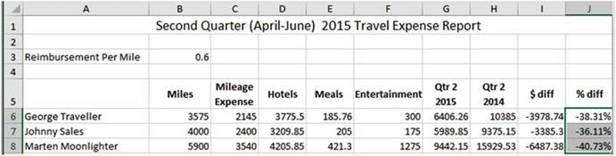
Figure 7-70.Add
two decimal positions to the cells
in the range J6:J8
17.
Press Ctrl + ~ to
view all the formulas on the worksheet. Press
Ctrl + ~ again to return to normal
view.

Mixed Cell References
Mixed cell Referencing is
a mixture of relative cell referencing and absolute cell referencing. Mixed cell referencing is when the row
is fixed but the column
is relative (the formula will be automatically adjusted to the column where the formula
is being copied
to) or vice versa.
Remember, in absolute cell referencing a dollar sign is placed
in front of both the column and row to lock them both. Mixed
cell references look like those in Table
7-4.
Table7-4.MixedCellReferences

Cell
Address�
Description
$A4���� The column remains the same, but the row can change when the formula is copied to another
location.
A$4���� The column
can change when the formula is copied to another location, but the row remains the same.
The dollar signs can be typed directly into the cell address or you can
place your cursor anywhere in the
cell address or one position to the left or
right of it and then press F4. This will create an absolute address
by placing
dollar signs in front of both the column and row such as $A$4. Pressing F4 a second
time places the
dollar sign in front of just the row, such as A$4. Pressing F4 a third time places
the dollar sign in front of the
column, such as $A4. Pressing F4 a fourth time removes the dollar signs thus returning the address to a
relative address.
Mixed cell referencing can best be illustrated by creating a table.
259
CHAPTER 7 ■ CREATING AND USING
FORMULAS
In this exercise we will create a
multiplication table that looks like Figure 7-71. The table could represent the
multiplication tables for numbers 1 through 7 or it could represent square
feet, the result of multiplying
length * width.
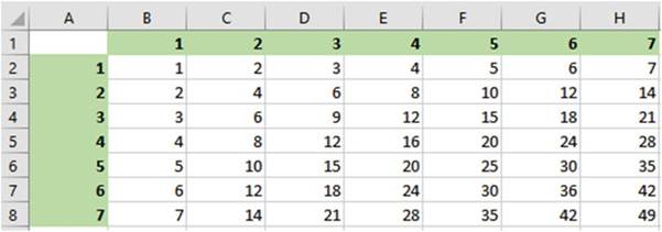
Figure 7-71. Multiplication table
1.
Create a new worksheet. Name the worksheet �Mixed.�
2.
Enter a 1 in cell A2. Enter a 2 in cell A3 and then press Ctrl + Enter.
3.
Drag across cells
A2 and A3. Use the AutoFill Handle
to copy the pattern down through row 8.
4.
Enter a 1 in cell B1. Enter a 2
in cell C1 and then press Ctrl + Enter
5.
Drag across cells B1 and C1. Use the AutoFill
Handle to copy the pattern
across through column
H.
6.
Bold the values you entered and give them a background color to
distinguish them.
7.
Enter =A2*B1 in cell B2. Press Ctrl + Enter.
8.
Drag the AutoFill
Handle down through
cell B8. Now drag the AutoFill Handle to the right to cell H8. Expand the width of the columns
so that you can see all the cell data. See Figure 7-72.
260
CHAPTER 7 ■ CREATING AND USING
FORMULAS
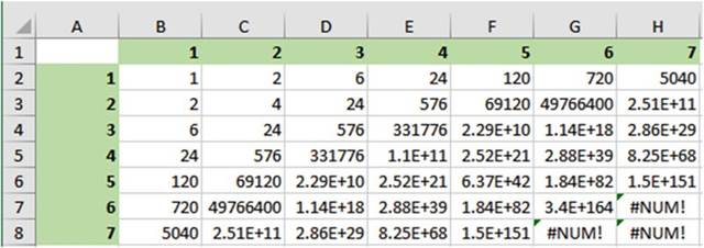
Figure 7-72.Results of multiplication using
relative cell addressing
This is definitely not the results we wanted. We wanted the spreadsheet to look like Figure 7-71.
9.
Press Ctrl + ~ to see the formulas. Your formulas should
look those in Figure 7-73.
Looking
at the formulas we can see that the columns have changed from the original
formula to adjust for the current column and the row address has changed to
adjust for the current row.
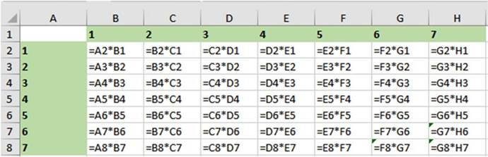
Figure7-73.Formulasusedinmultiplicationtable
When creating a mixed cell reference, you need to determine if it is the rows or columns
in the formulas that should remain constant.
In our example we want all of the formulas
to use column A. Therefore, we want the formula to lock in Column A. We need to make the first address in
the formula
in cell B2 $A2. Placing a $ in front of just the A will lock in the column but still allow the row in the
formula
to change to the current
row.
We want all the formulas to
use only row 1 but we want the column portion of the formula to change to the current column. Therefore we
need to lock in row 1 in the
second address in cell B2. Thus the
formula we need to use in cell B2 is =$A2*B$1.
10.
Double-click the address A2 in cell B2. Press
F4. The address should now be $A$2.
261
CHAPTER 7 ■ CREATING AND USING
FORMULAS
11.
Press F4 again.
The address is now A$2. Press F4 again. Your address should now
be $A2.
12.
Double-click the address B1 in
the formula. Press F4 twice. Your address should be
B$1. Press Ctrl + Enter.
13.
Drag the AutoFill
Handle down through
cell B8. Now drag the AutoFill Handle
to the right to cell H8. Your formulas should
look those in Figure 7-74. You can see that only column A was used in the formulas for the first
cell address and only row 1 was used in the second
cell address.
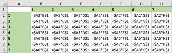
Figure7-74.Formulasusingmixedcellreferencing
14.
Press Ctrl + ~ to return to the results of the formulas. Your data should look like the table in
Figure 7-75.
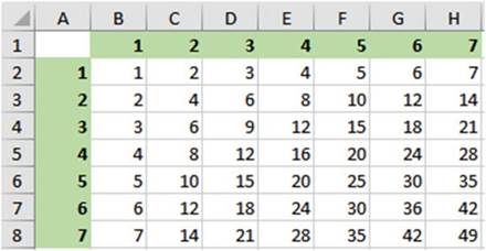
Figure7-75.Resultsofmultiplicationtable

You have
created formulas using absolute and mixed cell references. Knowing how and when
to use these are very important if
you want to become a skilled Excel user. Improper use of cell references is one
of the mistakes new Excel
students make most often. You should always review your formulas and their
results before relying on those
results.
262
Order of Precedence
CHAPTER 7 ■ CREATING AND USING
FORMULAS
The order of precedence is a set of predefined rules that determines the order in which operations in a
formula
will be performed. Looking at the formula
below it is difficult to know which operation to perform first.
= 3+2*18 /-3^2 � 2
Excel follows the normal Mathematical order of precedencealso known as the order of operations.
If an expression contains operators with the same precedence, they are evaluated from left to right. Placing
portions of the expression within parentheses allows you to control the order in which the operators are
evaluated. Excel performs mathematical operations in the order shown in Table 7-5.
Table 7-5. Order of Precedence
|
Operator
|
Description
|
Precedence
|
|
( )
|
Within parentheses
|
1
|
|
-
|
Unary operator (negative sign)
|
2
|
|
%
|
Percent
|
3
|
|
^
|
Exponentiation
|
4
|
|
*
|
Multiplication
|
5
|
|
/
|
Division
|
5
|
|
+
|
Addition
|
6
|
|
�
|
Subtraction
|
6
|
Now that you know the order in which
operations take place,
you can use this knowledge to determine the outcome of this formula.
=3+2*18/-3^2�2
Negative numbers
are evaluated first then Exponents. The expression is now equivalent to the following:
=3+2*18/9�2
Multiplication and division have the same level. Since the multiplication is to the left of the division, it
is
done first. The expression is now equivalent to the following:
=3+36/9�2
The division is performed next:
=3+4�2
Addition and Subtraction have the same precedence. Since
the addition is to the left of the subtraction, it is done first.
263
CHAPTER 7 ■ CREATING AND USING
FORMULAS
=7�2
The
subtraction is done next giving
a result of 5.
The normal operator precedence can be overridden by putting parentheses around the operations
you want performed first. If you have parentheses within parentheses, the operation in the innermost
parentheses is performed first.
The
formula could have been made clearer by the use of parentheses as in the formula that follows:
=3+((2*18)/(-3^2))�2
Summary
All formulas in Excel must start with an = sign.
Formulas can be entered
in one of three ways:
�
Typing directly into a cell
�
Clicking the cells
you want to reference in the formula
separated by mathematical symbols
�
Using your arrow
keys to select
the cells you want to reference separated by mathematical symbols
Excel follows the normal mathematical order of precedence. Be sure to use parentheses to make sure your
mathematical operations are performed in the order you want them to be.
Excel has an
Auto button that has the aggregate functions Sum, Average, Count, Min, and Max.
You don�t need to enter the
function to use one of these often used functions. Just select the cells above
or to the left of where you want to
place the result and then select the function you want to use by clicking the
down arrow to the right of the
AutoSum button.
You can assign a name to a range of cells. This can make your formulas easier to read and understand.
There are three places where you can name a range:
�
Name Box
�
Define Names dialog
box
�
Name Manager
Press Ctrl + ~
to display all of the functions on your worksheet. You can print your worksheet
with the formulas displayed. Press Ctrl + ~ again to display the results of your
functions rather than the functions themselves.
You can copy your formulas using
the Autofill Handle.
Any addresses used in your formulas will automatically adjust in the copied cells.
Addresses that adjust
are called relative
addresses. You can lock an address in a formula so that it will not adjust when being copied.
A locked address
is called an absolute address. The dollar sign is used to lock a row or a column. Press
F4 to place a dollar
sign in front
of the row and column.
If you lock only a row or only a column in an address
it is called a mixed
cell address.
You can select your named ranges and constants from a list by pressing F3.
You can place the names you assigned to ranges along with the range addresses in your worksheet by
clicking the down arrow to the right of Use in Formula and then selecting Paste Names. This creates
good documentation
for your worksheet.
264
CHAPTER
8
Excel�s Pre-existing Functions
This chapter covers
some of the most used functions that allow you to do such things
as sum values only if they
meet certain conditions, something based on whether a condition is true or not, determine the number of days
between
dates, get the current date and time,
and so on. You will learn how to enter
functions manually or by using
the Function wizard.
After reading and
working through this chapter you should be able to
�
Create a nested function
�
Use the Function wizard
�
Find the number of days between two days
�
Sum a range of values based on no
conditions, one condition, or multiple conditions
�
Get the month, day, or year from a date
�
Display different values based on whether a
condition is true or false
�
Get the integer portion of a decimal value
�
Get the current date and time and use them
in formulas
Excel�s Built-in Functions
Excel has lots of predefined built-in formulas which are called
functions. Each function has a unique name. The functions are grouped into categories. The function
categories are located on the Formula
tab�s Function Library group. Additional categories are available by clicking the More Functions
button. See Figure
8-1.
265
CHAPTER 8 ■ EXCEL�S PRE-EXISTING FUNCTIONS
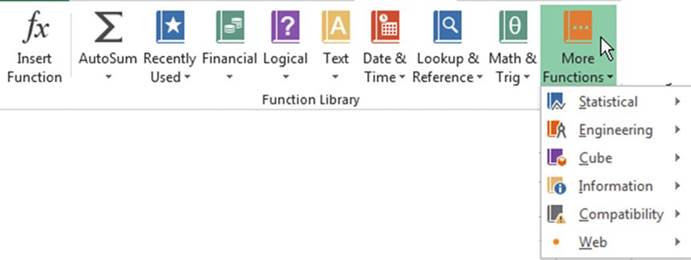
Figure8-1.Excelfunctionsarecategorized
Table 8-1 describes
the main built-in
functions.
Table8-1.FunctionCategoriesandTheirDescriptions

Function Category� Function Description
AutoSum������� The AutoSum
drop-down arrow displays
the �Auto� functions. These are the exact
same functions we looked at previously, and they are available on the Home tab in the editing
group. These functions
can return the sum, average,
count, highest value, and lowest value for a range of cells.
Compatibility����� These are functions that have been kept for compatibility with previous versions
of Excel. These functions have all been replaced with newer functions, so unless you need
backward compatibility you should not use them.
Cube������� These functions return
values from analysis
of multidimensional data sets used in
databases.
Date & Time����� Functions for dealing
with days, dates, and times Engineering����� Functions for engineering calculations
Financial����� Functions dealing with loans, investments, interest, depreciation, future
values, etc.
Information�����
Functions that help you determine the type of data that exists in a cell
Logical������ Logical functions are used primarily
in comparisons in which the result would be True or False.
Lookup &
Reference� Excel's Lookup &
Reference functions can be used to simplify
finding values in a list or data table or finding the reference of a cell.
Math & Trig���� Functions used for performing simple
and complex mathematical calculations Statistical����� Functions that perform
statistical analysis on ranges of data
Text��������� Functions
that manipulate text strings
Web�������� Gets data from a web service.
266
CHAPTER 8 ■ EXCEL�S PRE-EXISTING FUNCTIONS
The Recently Used button is not really
a category. It displays the last ten functions that you have used.
This creates a quick way to jump to some of the functions you probably use most often.
Function Construction
Each category consists
of separate functions
that relate to their category.
Figure 8-2 shows some of the Logical
functions.
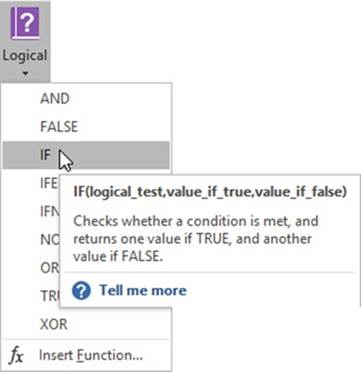
Figure 8-2. Logical functions
Moving your cursor over a function
provides a tool tip. The tool tip provides a description of the
function and its syntax. Each function has its own particular syntax.
Syntax is the rules for how a function can appear in a cell. Functions
usually contain arguments. Arguments are the values that are passed to the
function to work on. There are three arguments for the IF function (logical_test, value_if_true, and
value_if_false). Arguments are always separated
by commas. You would enter values or cell addresses
for the arguments. Clicking Tell me more will provide more help.
An example
of an IF function is =IF(C3>25000,C3*6%,C3*5%). The IF function
will be fully
explained later in this chapter.
Now that we have looked
at how a function is created we will look at the functions that you
are likely to use the most often.
Functions That
Sum Values
There are three functions for summing cell
values. Table 8.2 describes them.
267
CHAPTER 8 ■ EXCEL�S PRE-EXISTING FUNCTIONS
Table8-2.DescriptionsforSummingFunctions

Function� Description
SUM���
Sums a series of values without
testing for any conditions.
SUMIF��� Used to sum values provided
that they meet a condition that you specify.
SUMIFS�� Used to sum values only if multiple
conditions are met.

SUM
Function
We will look how a SUM function is constructed. The SUM function is one of the Math & Trig
functions. The SUM
function, used for
adding a group of values, is the most used function. The SUM function should be familiar to you, because
when you use AutoSum you are running the SUM function.
The Syntax for the Sum function is:
=SUM(number1, [number2], [number3]. . .)
Function names are written
in all capital letters; however,
they are not case sensitive. You could enter the
function name in small letters.
If you enter a function
in small letters
Excel will change it to all caps.
Function names are followed by a set of parenthesis. If the function requires arguments, they are placed
within the parenthesis. The SUM function has the arguments number1, number2 and number3. The arguments
number2 and number3 are placed within square brackets. Arguments placed within square brackets are optional.
The three dots (ellipsis) after the last argument mean that this is not the end of the list. You could
actually place any number of arguments within the parenthesis of the SUM function.
Excel is very helpful
when entering a function. As we saw in Chapter
7, entering a function in a cell starts by entering an = sign followed
by the name of the function. As you type the letters
of the function, Excel narrows
down the function
choices based on the letters
you have entered
so far. See Figure 8-3.
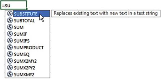
Figure 8-3.As you type the letters
of a function, Excel helps find a function that starts with those letters
Clicking a function name brings up a
description of what that function does.
After you have entered
enough characters to narrow down the function
to the one you want, press the Tab
key. Excel will place a left parenthesis after the function
name and it will bring up a tool tip to help you
with entering the function. The first argument
is highlighted in the tool tip. See Figure 8-4.
268
CHAPTER 8 ■ EXCEL�S PRE-EXISTING FUNCTIONS
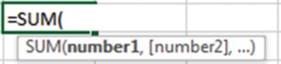
Figure8-4.Firstargumentishighlighted
After entering the first
argument and a comma (23, in this example), the second argument becomes highlighted in the tool tip and a
third
argument option is displayed. See Figure 8-5.
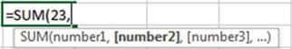
Figure8-5.Secondargumentishighlighted
Every time you enter another argument, an additional argument appears in the tool tip. See Figure 8-6.
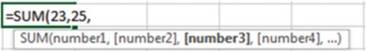
Figure8-6.Additionalargumentisaddedtotooltip
If you need to change one of the arguments you entered, click the argument
in the tool tip. This will select the argument
in the function and then you can make your changes. See Figure 8-7.
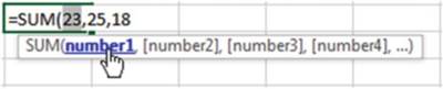
Figure8-7.Clickanargumentinthetooltip,toselectthatargumentinthefunction
You do not need to enter
a comma after
the last argument. It also is not necessary to enter the closing parenthesis. When you accept
the entry Excel
will automatically enter
the closing parenthesis for you. The result returned by the function will display in the cell where you
entered the function. The complete function
will display in the function
box. See Figure
8-8.
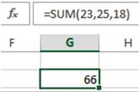
Figure 8-8.Result
of function appears
in the cell. The formula
for that cell displays in the Formula
bar
269
CHAPTER 8 ■ EXCEL�S PRE-EXISTING FUNCTIONS
Single values entered in a formula are
called constants. A constant
is a value that does not
change.
The entry for an argument
doesn�t have to be individual values like those
we have entered
in the SUM function. The SUM function can also use range names,
individual cell references, and cell ranges
for its arguments.
What can be entered for each argument
depends upon the function used.
Table 8-3 shows several examples
of the SUM function with different arguments.
Table8-3.TheSUMFunctionwithDifferentArguments

Function��� Description
=SUM(3,5,8)�� Adds the individual values 3, 5 and 8 giving a result of 16
=SUM(Sales)� Adds the values in the range named Sales
=SUM(B3:B9)� Adds the values
in the range B3 to B9

If you wanted
to sum the cells in the range
C5 to C10 on a different worksheet named �Purchases,� you would enter the formula
as shown in Figure 8-9.
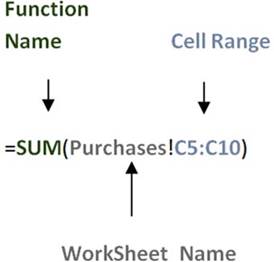
Figure 8-9.Using the SUM function to sum a range
on a different worksheet
You could
type Purchases! or you could
click the worksheet named Purchases and Excel would
enter the name along
with the exclamation point in the formula for you.
If you only wanted
to add the values in column C, then you could use the shortcut
method C:C. The formula could be written
as =SUM(Purchases!C:C)
Using the Insert
Function Option
As we discussed in Chapter 7, clicking
the Insert Function
button in the Function
Library group brings
up the Insert Function dialog
box See Figure
8-10.
270
CHAPTER 8 ■ EXCEL�S PRE-EXISTING FUNCTIONS
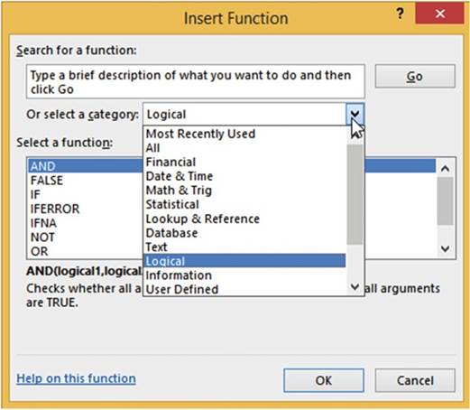
Figure 8-10. Insert Function dialog box
Clicking the down arrow for the Or select a category list box brings up the same categories that are
available
in the Function Library group. The only additional category
here is the All category.
If you don�t know the category
for the function you want to use, clicking the All category
will bring up every function from every category in alphabetical order. The syntax and description for each
function
appears as you click
the different functions,
A primary reason
for using the Insert Function
option is for its search
capability. You can type a description of what you want a function to do into the search
text box and then click
the Go button. Excel will provide a list of functions that may meet your needs.
In Figure 8-11, �find
the largest number�
was entered for the search.
Excel returned with a list of functions that would meet that criterion. It would be up to you then to decide
which one in the list best meets
your needs.
271
CHAPTER 8 ■ EXCEL�S PRE-EXISTING FUNCTIONS
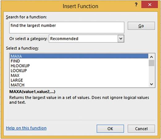
Figure 8-11.Enter what you want to do in the Search
for a function text box and then Excel attempts
to find a function that meets your needs
We will add three columns of numbers using the SUM function.
1.
Create a new workbook. Enter
the data in Figure 8-12 into a worksheet. Name the worksheet �Sum.�
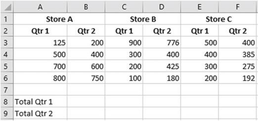
Figure8-12.Enteryourdatainaworksheetinthisformat
272
CHAPTER 8 ■ EXCEL�S PRE-EXISTING FUNCTIONS
2.
Click inside cell B8. On
the Formulas tab in the Function Library group click the Insert Function button.
3.
Enter add numbers in
the Search for a function
box. Press Enter or click the Go button. Click SUM in the Select a function list box. Click the OK
button. See Figure 8-13.
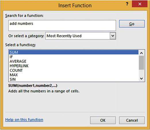
Figure 8-13. Searching for a function
4.
The Function Arguments dialog box opens.
Move the dialog
box if it is covering the numbers
in your worksheet. An entry box appears for each required
argument.
Click inside the Number1 box. Required arguments
are bolded. Number1
is the only required argument
for the Sum function.
See Figure 8-14.
273
CHAPTER 8 ■ EXCEL�S PRE-EXISTING FUNCTIONS
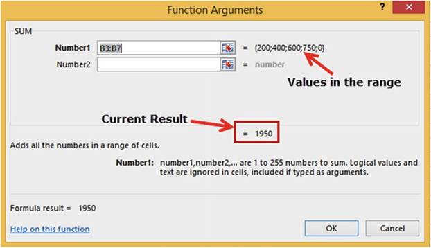
Figure 8-14.Excel
assumes you want to add the cell range B3:B7 and enters
the range for the first
argument
Argument Number1
contains the range B3:B7 because
it is attempting to add the values above it. The values
being summed are displayed to the right of the Number1 box. It includes
the 0 for cell B7. This doesn�t
affect the current
total, which as you can see is 1950.
5.
Drag across cells
A3:A6. The values
from this range
are displayed as well as the current
sum. See Figure
8-15.
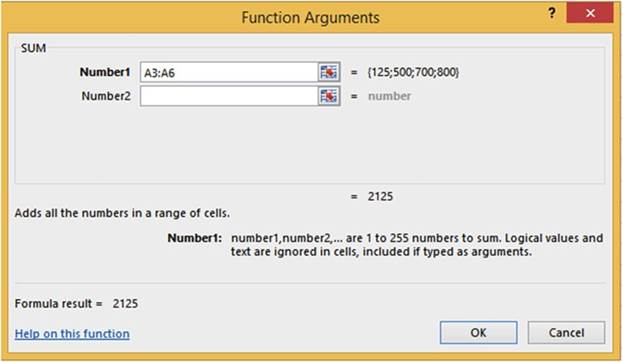
Figure8-15.ExcelsumsthevaluesintherangeA3:A6
274
CHAPTER 8 ■ EXCEL�S PRE-EXISTING FUNCTIONS
6.
The Collapse Dialog
 �buttons can be used to collapse
the window when it is blocking the data you need to use. Click
inside the Number2
box. Click the
�buttons can be used to collapse
the window when it is blocking the data you need to use. Click
inside the Number2
box. Click the
 �button to the right of the Number2 box. The window
collapses to a single box for the current argument.
Drag across cells C3:C6. See Figure 8-16. When you have finished your selection click the Expand
Dialog
�button to the right of the Number2 box. The window
collapses to a single box for the current argument.
Drag across cells C3:C6. See Figure 8-16. When you have finished your selection click the Expand
Dialog
 �button to expand the window back.

Figure 8-16. Collapsed Window
7.
The Number3 argument has been added to
the window.
Click
inside the Number3 box. The Number4 argument has been added. Drag across cells E3:E6. Figure 8-17 displays
the result. Click the OK button.
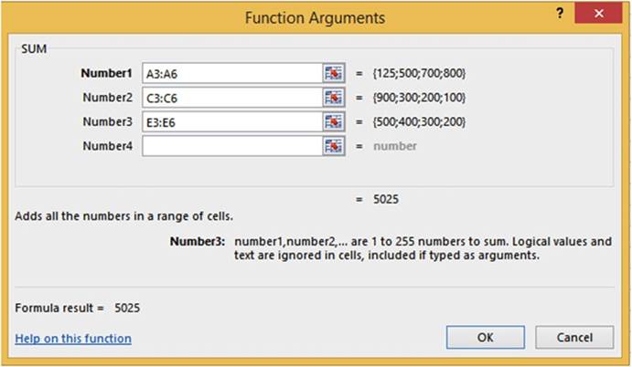
Figure 8-17.Additional arguments were added. The first three arguments have been
added
and the result
is 5025
The result is placed in cell B8.
Using the same steps see if you can
get the answer for cell B9.
275
CHAPTER 8 ■ EXCEL�S PRE-EXISTING FUNCTIONS
You have learned
how to add all of the values
in a single range or in multiple
ranges at the same time.
What if you only want to add only some of the values in a range such as expenses, but only if they are
entertainment expenses?
You�ll see how to do this in the next section.
SUMIF�Adds the Cells That Meet a Specified
Criteria
The SUMIF function is used for summing
a range of values provided
that they meet a condition that you specify in the criteria
argument. The SUMIF function
only works if you are basing your summing on a single criterion. If you need to base it on more than one
criterion you will need to use the SUMIFS function,
which is covered
in the next section.
The syntax for the SUMIF function is:
SUMIF(range, criteria, [sum_range])
Argument descriptions are
range is the cells
that you are basing your criterion on. The range
contains the values that will be checked by the criteria
to determine if they are to be included in the sum.
criteria is the condition
that must be met if a value is to be included
in the sum. If the condition contains
any text, logical
or mathematical symbols
it must be enclosed in double quotation
marks. Quotation marks are not necessary if the criterion
is just a number.
[sum_range] is optional. If this optional
range is used then it will be this range that contains
the cells to be summed
rather than the range in the first
argument. The criteria
will still be based on the first
range argument.
Using SUMIF with the Required Arguments
Figure 8-18 contains
a range of values that need to be summed,
but we only want to sum those
items whose value is greater
than 900. There
are only two values greater
than 900 in the range
B1:B6: 1100 and 1500.
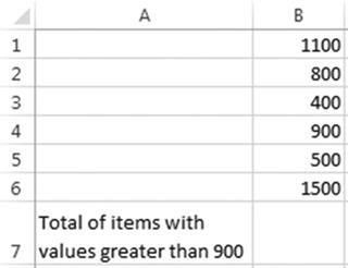
Figure 8-18.The
values that are greater than 900 will be summed
276
CHAPTER 8 ■ EXCEL�S PRE-EXISTING FUNCTIONS
The arguments used in the formula for summing the values greater
than 900 are
B1:B6 is the range
of values that the criteria
will be based
on.
">900" is the criteria. Since the criterion contains something
other than just a number it must be
enclosed in double quotes.
The complete formula is =SUMIF(B1:B6,">900").
We will place
this formula in cell B7. The result
of adding 1100 + 1500 is 2600.
See Figure 8-19.
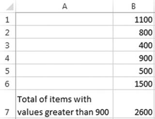
Figure 8-19. Result of SUMIF function
Figure 8-20 shows a list of items
and their prices.
We only want to sum those items
whose price is exactly 99 cents. The formula entered
into cell B10 is =SUMIF(B2:B8,0.99). Since we are only summing those values which
are exactly .99, there is no need for any additional logical
symbols because the equal sign is optional.
Because the criterion is only a number, it does not need to be placed
within double quotes.
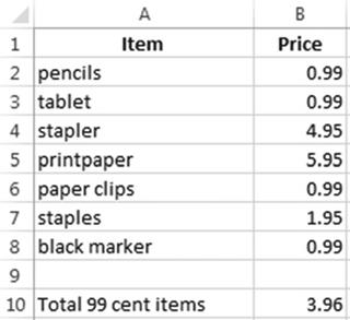
Figure8-20.Sumofthefour.99prices
277
CHAPTER 8 ■ EXCEL�S PRE-EXISTING FUNCTIONS
Using the Optional
sum_range Argument
When using the optional sum_range argument you base your criteria
on a different range of cells than those
that you are summing.
We want to find the total
number of males
and females in a high school. Figure
8-21 shows the worksheet for this. The worksheet uses separate formulas
for determining the number of males and females. The arguments used in the formula for determining the
number of males are:
B2:B9 is the range that the criteria
will be based on.
"�M" is the criterion
C2:C9 is the sum_range. The range of the cells that will be summed,
if the criterion is met.
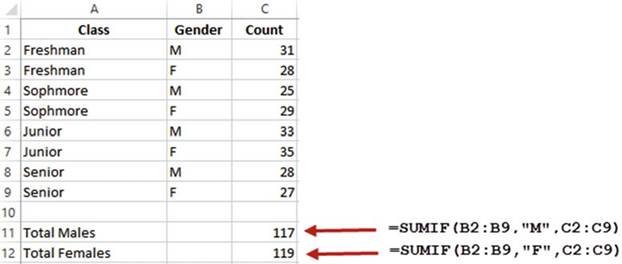
Figure 8-21. Result of SUMIF functions
The formula entered in cell C11 is
=SUMIF(B2:B9,"M",C2:C9)
The only difference in the formula
for computing females
is the criterion which is "F". The formula
entered in cell C12 is
=SUMIF(B2:B9,"F",C2:C9)
SUMIFS�Adds the Cells
That Meet Multiple
Criteria
The SUMIFS function
is similar to the SUMIF function
except that the SUMIFS function is used to sum values only if multiple
conditions are met rather than a single
condition.
The syntax for the SUMIFS function is:
SUMIFS(sum_range, criteria_range1,
criteria1, [criteria_range2, criteria2], . . .)
278
CHAPTER 8 ■ EXCEL�S PRE-EXISTING FUNCTIONS
Argument descriptions are
sum_range is the cells that you are basing your criteria
on. The range contains the values that will be checked by the criteria
to determine if they are to be included in the sum.
criteria_range1 is
the first range in which to evaluate the associated criteria.
criteria1 is the condition that defines which cells in
the criteria_range1
argument will be added.
Criteria_range2, Criteria2,. . . You can add as many as 126 additional
ranges and their associated criteria.
Figure 8-22 shows a company�s bank deposits along
with the date of each deposit for its different branches. We want to sum the bank deposits
in column B but only if the following conditions are met:
�
It is not a Hobart office.
�
The amount of the deposit has to be at least
20,000.
�
The date of the deposit
has to be 03/12/2010 or later.
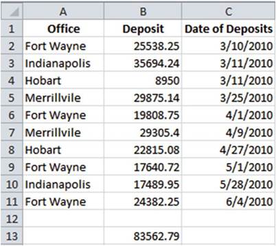
Figure 8-22. Result of SUMIFS function
The formula that will add the deposits that
meet our criteria is:
=SUMIFS(B2:B11,A2:A11,"<>Hobart",B2:B11,">=20000",C2:C11,">=03/01/2010")
The arguments used in the formula for summing the bank deposits are as follows:
B2:B11 is the sum_range. This range contains
the values we want to sum if they
meet our criteria
279
CHAPTER 8 ■ EXCEL�S PRE-EXISTING FUNCTIONS
We only want the branches that are not
Hobart.
�
A2:A11 is the criteria_range1.
�
"<>Hobart" is criteria1.
The amount of the deposit has to be at least
20,000.
�
B2:B11 is the criteria_range2.
�
">=20000" is criteria2.
The date of the deposit
has be 3/12/2010 or later.
�
C2:C11 is the criteria_range3.
�
">=03/12/2010" is criteria3.
Figure 8-23 highlights
the rows that meet all the criteria.
They are the only deposits
that meet all three criteria
of (1) not being a Hobart branch,
(2) having a deposit greater
than or equal to 20000, and (3) having
been deposited on or after 3/12/2010. The result of adding the deposit for these three rows is 83562.79
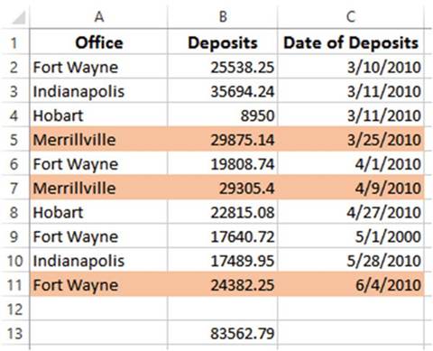
Figure8-23.RowsthatmeettheSUMIFScriteriaarehighlighted
Using a Cell Address
Rather Than a Cell Value for a Criteria
If you are checking if an item is equal to a value in the criteria
range you can specify a cell address
that contains the value of that item for the criteria. In Figure 8-24 we want to sum the attendees if they
took an Excel class in Fort Wayne. Cells E2 and F2 can be used for the criteria
because they contain
the values to be checked
against the criteria
range.
280
CHAPTER 8 ■ EXCEL�S PRE-EXISTING FUNCTIONS
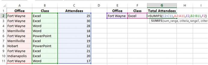
Figure8-24.ThecriteriaforSUMIFSisincellsE2andF2
Figure 8-25 shows the formula entered in cell G2.

Figure8-25.BreakingdowntheSUMIFSformula
Handling Empty Cells in SUMIFS Functions
The worksheet in Figure 8-26 totals the values
for items that have been completed but haven�t yet shipped.
The two criteria that will be used for the SUMIFS arguments will be those items whose Date Completed
is not blank and whose Date Shipped is blank.
The figure highlights those items that meet both criteria.
281
CHAPTER 8 ■ EXCEL�S PRE-EXISTING FUNCTIONS
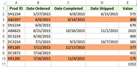
Figure 8-26.Rows
are highlighted where the items have been completed but not shipped
The criteria are as follows:
The criteria for the Date Completed cells is
"<>"
The criteria
for the Date Shipped is "" (two quotes together
test for a blank) The formula entered
in cell E11 is =SUMIFS(E2:E10,C2:C10,"<>",D2:D10,"").
■
Note� When testing a criteria range for blanks the cells must be real blanks and
not the result of a formula that had no result.
IF�Returns Different Values Depending upon If a
Condition Is True or False
The IF function returns different values depending upon whether a condition is true or false.
The syntax for the IF function is:
IF(logical_test , [value_if_true],
[value_if_false])
Argument descriptions are
logical_test is
the condition being tested.
[value_if_true] if
the condition being tested is true, then perform this step.
[value_if_false] if the condition being tested is false, then perform this step.
If the condition being
tested is true, what is in the value_if_true argument will be used; otherwise what is in the value_if_false
argument will be used.
Let�s say that the value in cell A2 is 20. If you place the following formula
in cell A1
=IF(A2=20,"Equal 20","Not equal 20")
282
CHAPTER 8 ■ EXCEL�S PRE-EXISTING FUNCTIONS
then cell A1 will display Equal 20. If you change the value in cell A2 to 19, then the value in cell
A1 will change to Not equal 20.
We need to determine the
Gross Pay for each of our employees. If an employee works over 40 hours he will receive overtime
pay at 1.5 times the normal rate. The Gross Pay will be computed by adding an employee�s
regular pay and overtime pay.
An IF function will be used to compute the employee�s regular pay; another IF function will be used to
compute his or her
overtime pay.
If an employee works 40 hours or less, his regular pay and his gross pay would
be the hours he worked times his pay
rate.
If an employee
works 40
hours or
more, then his regular pay will
be 40
hours times
the pay
rate. The
hours the employee worked
in addition
to the
40 hours
will be
used for
determining overtime pay. If we assign
names to
our ranges,
the formula needed to
compute regular pay is =IF(hours>40, 40*rate, hours*rate).
We take 40 * rate if the condition (hours
>40) is true and hours * rate if
the condition is false.
To compute
the OT (overtime pay) we will again need to test if the hours worked is greater
than 40.
If the hours are greater than 40 we will need
to take the number of hours worked minus 40 to get the overtime hours. The
overtime hours will be multiplied by the pay rate times 1.5. If the hours worked are 40 or less, then the
overtime will be 0.
Figure 8-27 shows the formula to compute the overtime pay.
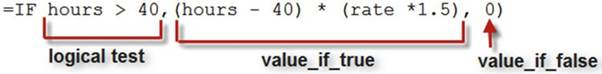
Figure 8-27. The overtime pay formula
1.
Enter the data in Figure 8-28 in a new worksheet. Name the worksheet �Payroll.�
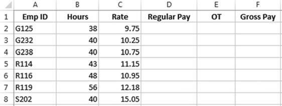
Figure8-28.EnterthisdatainanewworksheetnamedPayroll
283
CHAPTER 8 ■ EXCEL�S PRE-EXISTING FUNCTIONS
2.
Select the range B1:E8, as in Figure 8-29.
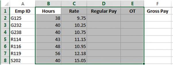
Figure 8-29. Select range B1:E8
3.
On the Ribbon click the Formula tab. In the Defined Names
group click the Create from Selection button. Select Top row from the Create
Names from Selection dialog box. See Figure 8-30.
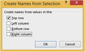
Figure8-30.SelectToprowintheCreateNamesfromSelectiondialogbox
4.
Type
this formula in cell D2: =IF(hours >=40,40*rate,hours*rate).
Press the Tab key.
5.
Type
this formula in cell E2: =IF(hours > 40,(hours - 40)*rate* 1.5,0). Press the Tab key.
6.
Type this formula
in cell F2: =Regular_Pay+OT. Press the Enter key.
7.
Select the range D2:F2. Drag
the AutoFill Handle down through row
8. Figure 8-31 shows
the result.
284
CHAPTER 8 ■ EXCEL�S PRE-EXISTING FUNCTIONS
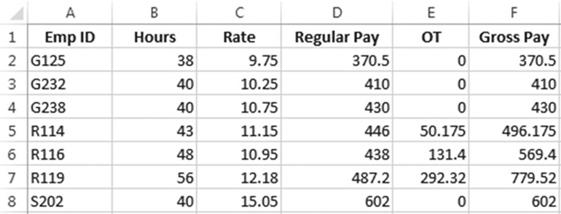
Figure8-31.ResultofcopyingformulaswithAutoFillHandle
8.
We need to change the Regular Pay, OT, and Gross Pay columns so
that they display with two decimal positions. We also want to show dashes instead of
zeroes for the overtime pay. Formatting the cells as the Accounting type will do this for us.
a.
Select cells D2:F8.
b.
Right-click the cells and then select Format Cells.
c.
Select the Number tab.
d.
Select Accounting for the Category. Click the down arrow
for the Symbol
and then select
None.
e.
Click the OK button. Figure 8-32 shows the results.
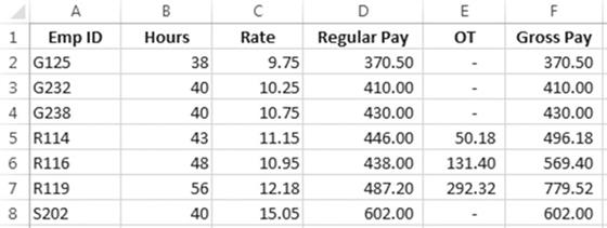
Figure8-32.ResultofformattingtherangeD2:F8asAccounting
You have used the IF statement to test a condition; the function does one thing if the condition is true
and something else if the condition is false. Next, you will look at the AND function and later the OR
function. These functions don�t do much on their own. They only return
either a TRUE or FALSE.
Their strength is shown when they are combined with other functions. The exercise following
the OR function demonstrates how to combine
these functions within
an IF function.
285
CHAPTER 8 ■ EXCEL�S PRE-EXISTING FUNCTIONS
AND - Returns TRUE if
All of Its Arguments Are TRUE
The AND function returns either a TRUE or a FALSE.
It returns a TRUE if all
of its arguments are
true and it returns a FALSE if any of
its arguments are not true.
The syntax for the AND function is:
AND(logical1, [logical2], . . .)
The AND function can be used to evaluate up to 255 logical conditions.
Figure 8-33 shows the AND function
with three logical
conditions. All three
of these conditions are true therefore
the function returns
a TRUE.
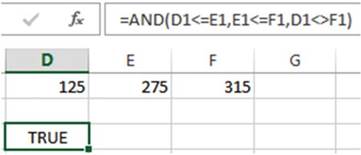
Figure8-33.ANDfunctionthatteststhreeconditions
The last condition in Figure 8-34 is false. The value in cell D1 is not equal to the value in cell F1. The
AND function therefore returns
a FALSE because
even if only one of the logical
conditions is false it will return a FALSE.
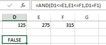
Figure8-34.Thethirdconditionisfalse,whichreturnsafalse
OR�Returns TRUE If Any Argument
Is TRUE
The OR function returns a TRUE if any of its
arguments are true and it returns a FALSE if all of its arguments are false.
The syntax for the OR function is:
OR(logical1,[logical2],. . .)
286
CHAPTER 8 ■ EXCEL�S PRE-EXISTING FUNCTIONS
Figure 8-35 shows the OR function with three logical conditions. All three of these
conditions are false. If and only if all
of the arguments are
false will the OR function return a FALSE.
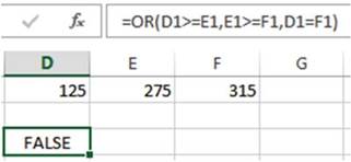
Figure8-35.AllconditionsarefalsesotheORconditionreturnsaFALSE
The first
logical condition in Figure 8-36 is true. The value in cell D1 is less than the value in cell E1. The
other conditions are false. The OR function returns a TRUE because
even if only one logical
condition is true the function
returns a TRUE.
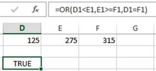
Figure 8-36.Only
the first condition is true; therefore, the OR function
returns a TRUE
Nested Functions
Sometimes
a single function
will not give you the results you need. In these cases you will need to create a nested function.
Nested functions combine
the operations of two or more functions
into a single function. A nested function
is used as an argument
in the other function. Excel allows a maximum of 64 functions
nested within each other. That should be more than you will ever need.
287
CHAPTER 8 ■ EXCEL�S PRE-EXISTING FUNCTIONS
In this exercise you create functions nesting different operators.
Nesting
an AND function Within an IF Function
1.
Enter the data in Figure 8-37 into a worksheet. Name the worksheet �Nested.�
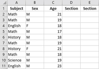
Figure8-37.EnterthisdatainaworksheetnamedNested
Students who are in Math,
are males, and are less than 21 years old will be placed in Section A. This problem
will require an AND function nested
within an IF function.
The AND function will be the condition to be tested.
If the condition is true we will display an A in the cell.
If the condition is false
we will display a blank.
2.
Select the cell range A1:C11. On the Ribbon�s Formula
tab in the Defined Names group click Create
from Selection. In the Create Names from Selection window,
only Top row is to be selected. Click the OK button.
3.
Click the down arrow of the name box to see your named ranges.
4.
Click inside cell D2. Start
the formula by entering =IF(AND( The Excel tool tip shows the needed arguments for the AND function. See
Figure 8-38.
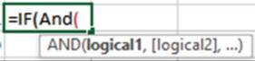
Figure 8-38. Tool tip for the AND function
288
CHAPTER 8 ■ EXCEL�S PRE-EXISTING FUNCTIONS
5.
We will now enter the first of the three conditions we will be testing
for.
a.
Press F3 to bring up the range names. Select Subject and then click the OK button.
b.
Enter ="Math" followed by a comma. Entering
the comma highlights the second argument
[logical2]. See Figure
8-39.
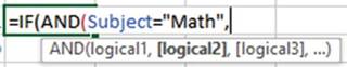
Figure8-39.Enteringacommainthefunctionhighlightsthenextargumentinthetooltip
6.
Press F3 to bring up the range
names. Select Sex and then click the
OK button.
7.
Type ="M",. The formula should now be
=IF(AND(Subject="Math",Sex="M",
8.
Press F3 to bring up the range names. Select Age and then click the OK button.
9.
Enter
<21), The formula should now be =IF(AND(Subject="Math",Sex="M",A
ge<21),
The AND function is finished
and now you are back to the IF function and ready to enter the data for the argument [value_if_true]. See
Figure
8-40.
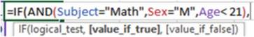
Figure 8-40.The AND function
is completed; [value_if_true], is highlighted to let you know that you should now enter this argument
for the IF function
10.
Enter "A", for the true argument. Enter "") for the false argument. This will
display a blank.
The complete formula is =IF(AND(Subject="Math",Sex="M",Age<21),
"A","").
If you didn�t enter "" for the false part
Excel would by default display the word False.
11.
If you wanted to see or make a change to your formula you could click the
word IF
and then
click the Insert Function button (Formula tab | Function Library).
You can see
that the AND condition is
false; therefore our result is a blank. See
Figure 8-41.
289
CHAPTER 8 ■ EXCEL�S PRE-EXISTING FUNCTIONS
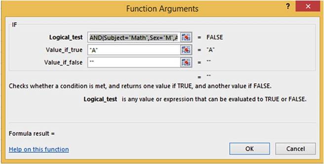
Figure 8-41.The
Function Arguments dialog
box shows the results of the Logical_test
12.
Click the Cancel button.
13.
If you just wanted to see or make a change to the AND function you could click the word AND
and
then click the Ribbon�s Formula
tab. In the Functions Library
group click the Insert Function
button. See Figure 8-42. You can see that the Age is not less than 21 for the first cell in the range.
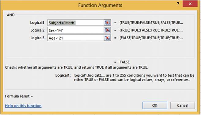
Figure8-42.Theresultofthelogicalargumentisshownforeachcell
290
CHAPTER 8 ■ EXCEL�S PRE-EXISTING FUNCTIONS
14.
Click the Cancel button.
15.
Press Ctrl + Enter to accept the formula.
Cell D2 is blank.
16.
Use the Autofill Handle to copy
the formula from D2 to D11.
Nesting an
OR Function Within an IF Function
Let�s create another IF function, but
this time let�s nest an OR function within it that will test if the student is a female or if the
student is 21 or more. If a student
meets either one of these conditions, he or she will be placed in Section B.
1.
In cell E2 enter the formula =IF(OR(.
2.
Press F3 to bring up the range
names. Select Sex and then click the
OK button.
3.
Type Sex
= "F",.
4.
Press F3 to bring up the range names. Select Age and then click the OK button.
5.
Type Age
>= 21),. The function is now =IF(OR(Sex="F",Age>=21),.
The OR function is finished
and now you are back to the IF function and ready to enter the data for the argument [value_if_true]
6.
Enter "B","").
The full formula is =IF(OR(Sex="F",Age>=21),"B","").
7.
As with the nested AND function, clicking the word IF in the formula and then clicking
the Insert Function or clicking the word OR
in the formula will display that portion of the formula in the Function Arguments window.
8.
Use the Autofill
Handle to copy the formula
from E2 to E11. Select
the cell range B2:E11. Center
the data of the selected
range. Figure 8-43 shows the results.
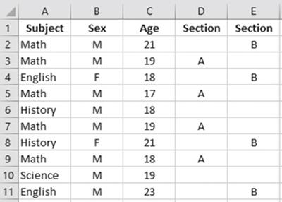
Figure8-43.RangeB2:E11centeredincells
291
CHAPTER 8 ■ EXCEL�S PRE-EXISTING FUNCTIONS
Let�s make a change to the application by placing a check mark in column D if the student
meets the conditions of being a Male, a History major,
and under 21. The check mark is part of the Wingding
font Set. A check mark is created
when you hold your Alt key and then on the numeric
keypad type 0252 (it only works if you use the numeric
keypad). The Wingding
font must then be selected
for the cell.
9.
Delete column E.
10.
Change the text in cell D1 to Section A.
11.
Click cell D2. In the Formula bar select A in the true part of the IF formula.
12.
Hold
down the Alt key and type 0252 on the numeric keypad. The formula should be
=IF(AND(Subject="Math",Sex="M",Age<21),"�","")
13.
Select the Autofill handle on
cell D2 and drag it down through cell D11.
14.
With the range
D2:D11 selected, change the Font
typeface to Wingdings. Figure 8-44 shows
the result.
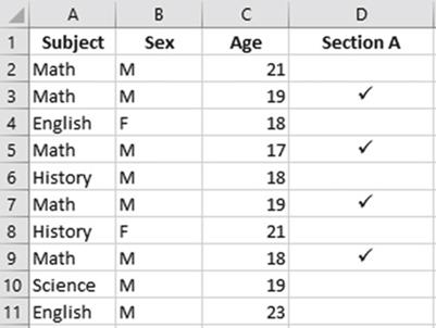
Figure8-44.UseWingdingstocreatecheckmarks
You created nested AND and OR functions. You can nest about any function within another. This gives
your functions a lot more flexibility. Next, you will look at functions that deal with dates. You�ll see how
you
can get the current date and time, find the number of days between
two dates, and manipulate dates by adding or deleting
from them.
Date Functions
Excel allows you to use dates and times in formulas. Excel
can do this because it actually stores
dates and times as numbers.
Excel stores dates
as serial numbers.
A serial number
treats January 1, 1900 as the first
day of the calendar. It is considered as day 1. January 2, 1900 is considered day 2, January
3, 1900 is considered day 3, etc. Because Excel
treats January 1, 1900 as the first
day you can�t
use any dates
earlier than this.
If you do, Excel will treat the date as text.
292
CHAPTER 8 ■ EXCEL�S PRE-EXISTING FUNCTIONS
You can see how Excel treats dates and times
by formatting them as General.
In the example in Figure 8-45, 1/1/1900
was entered in both cells A1 and B1. The date 3/2/1010
was entered in both cells A2 and B2. Cells B1 and B2 were formatted
as General.
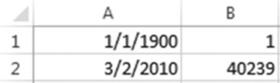
Figure 8-45.Column
B shows what the date in column A looks like when formatted as General
Cell B2 displays
40239, which is the number
of days between
1/1/1900 and 3/2/2010.
Excel stores times as a value between 0 and 1. The time 12:00 AM would be stored as a value of 0. The
time 11:59:59 PM would be stored as a value of .9999.
TODAY Function�Returns the Current Date
The TODAY() function returns the current date, which it gets from your computer�s
internal clock. The TODAY() function doesn�t use any arguments.
Even though the TODAY function doesn�t use any arguments you must still enter parentheses after the function
name so that Excel recognizes it as a function.
The syntax for the TODAY function is:
=TODAY()
See Table 8-4 for some examples.
Table8-4.DescriptionandResultsforVariousTODAYFunctionFormulas
|
Formula
|
Description
|
Result if today was 10/11/2015
|
|
=TODAY()
|
Returns
the current date
|
10/11/2015
|
|
=TODAY() + 10
|
Returns
the date ten days into the future
|
10/21/2015
|
|
=TODAY()
� 5
|
Returns
the date five days ago
|
10/06/2015
|
The TODAY() function is recalculated every time you open the worksheet or refresh it. In other words, if you
enter the formula =TODAY() in a worksheet on May 01, 2016 and then reopen that same worksheet on June 30,
2016 the date will be updated to 06/30/2016. You can prevent this dynamic updating by making the date
static.
To make the date
returned from the TODAY()
function static
1.
Double-Click
the cell that contains the Today() function. This
places the cell in edit mode.
2.
Press the refresh key (F9). This changes the date to a serial date. See Figure 8-46.

Figure8-46.Thedatedisplayedasaserialdate
293
CHAPTER 8 ■ EXCEL�S PRE-EXISTING FUNCTIONS
3.
Press Enter
to commit the entry. The serial number
then reverts back to a date
format. The date will then always show as the date you made the entry.
In this exercise you will you use the TODAY function and a person�s birthdate to determine his or her age.
1.
Enter the data in Figure
8-47 in a new worksheet. Name the worksheet �Age.� We want to determine the age for those whose
birthdate appears in column B. Add your name and birthdate to the list.
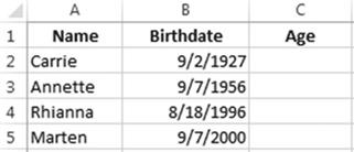
Figure8-47.EnterthisdatainaworksheetnamedAge
2.
Click inside cell C2. The formula for determining the age is today�s date minus the birthdate
divided
by 365.25. We divide by 365.25 to accommodate leap year which happens every
four years.
3.
Type =(TODAY()-B2)/365.25.
We place a pair of parentheses around TODAY()-B2
because we need to perform
this calculation before doing the division. If
we didn�t place it in parentheses Excel would first divide B2 by 365.25.
4.
Press Enter. The result is a decimal
amount. We usually
display someone�s age as an integer.
We will use the INT function
to remove the decimal portion of the age. The
INT function rounds a value down to its nearest whole number
5.
Double-Click cell C2.
6.
Place the cursor after the equal sign in the Formula bar. Type INT(.
7.
Press the End key on the keyboard to place the cursor at the end of the
function.
8.
Type the closing right parenthesis. Your
formula should now be
=INT((TODAY()-B2)/365.25)
9.
Press Ctrl + Enter.
10.
Drag the AutoFill
Handle down through cell C5. If this
was run in February 2016 the results
would be as shown in Figure 8-48.
294
CHAPTER 8 ■ EXCEL�S PRE-EXISTING FUNCTIONS
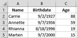
Figure8-48.ResultofusingTODAYfunctionwithINTfunction
NOW Function�Returns the Current Date and Time
The NOW function is similar to the TODAY function except that the NOW function includes the time along with
the current date. Another difference is
that the NOW function is not dynamic. It does not update to the current date when you reopen the worksheet.
The syntax for the NOW function is
=NOW()
Table 8-5 shows an example
of the NOW function applied on October 20, 2015 at 3:18 PM.
Table 8-5. NOW
Applied

Formula�� Displays
current date and time
=NOW()�� 10/20/2015 15:18

Notice that the NOW function displays time in a 24-hour format.
You can change
the Time format
so that it will display in a 12-hour
format using AM or PM. Changing the time to a 12-hour
format requires a custom
format. This date and time
 �is the result of entering
=NOW() in a cell. To change to a 12 hour format that displays AM or PM you would
right-click the cell and select Format. This would bring up the Format Cells dialog box. See Figure
8-49. Make sure that Custom is selected
for the Category and m/d/
�is the result of entering
=NOW() in a cell. To change to a 12 hour format that displays AM or PM you would
right-click the cell and select Format. This would bring up the Format Cells dialog box. See Figure
8-49. Make sure that Custom is selected
for the Category and m/d/
yyyy h:mm is selected for the Type
295
CHAPTER 8 ■ EXCEL�S PRE-EXISTING FUNCTIONS
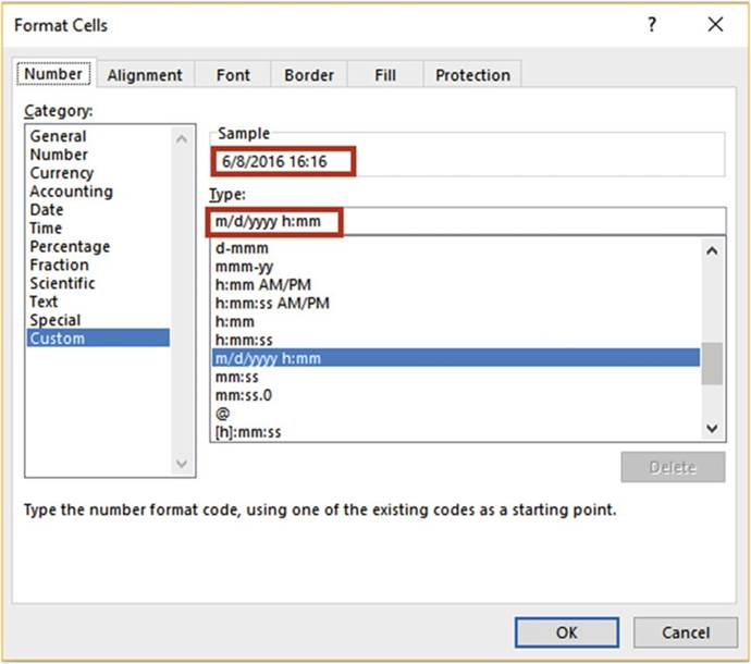
Figure 8-49.Select
the Custom category
and the date and time type
You would
then add AM/PM
to the end of the type. See Figure 8-50. The result is shown in the Sample area. You would then click the OK
button
and the cell would display
the same value
as what appears
in the Sample area.
296
CHAPTER 8 ■ EXCEL�S PRE-EXISTING FUNCTIONS
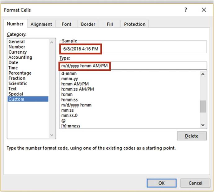
Figure 8-50.Adding AM?PM changes the time from a 24-hour format to a 12-hour format
that shows AM or PM
If you just wanted to display the time
without the date you could use the following formula:
=NOW() � TODAY()
DATE Function�Returns the Serial Number
of the DATE
The DATE function returns the serial number of the
date provided in the DATE
arguments.
The syntax for the DATE function is:
=DATE(year, month, day)
297
CHAPTER 8 ■ EXCEL�S PRE-EXISTING FUNCTIONS
All of the arguments in the DATE function
are required.
When you create a new workbook
all of the cells are formatted as General by default. If you enter
the formula =DATE(2015, 10, 20) Excel will automatically change the formatting of the cell to the date type
and
display 10/20/2015. The date is actually stored
as a serial number so that it can be used in formulas. If you format
the cell as something other
than a date or time,
Excel will display
the date as a serial
number. Remember, the serial number
is the number of days that have passed since
January 1, 1900.
■
Note� You should always enter a four-digit year when using the DATE function.
If you enter a one- or two-digit year Excel will treat these as from the
1900s. For example, if you enter =DATE(09,05,14) or
=DATE(9,05,14) Excel will
assume the year is 1909 not 2009.
The DATE function is most useful in situations in which you are getting the year, month, and day from other
cells or when you want to use the date as part of a formula. You can�t enter a date directly in a formula.
If you enter a formula as =09/07/2015�09/05/2015 Excel treats the forward slashes as divide signs. If you
want to use a date in a formula you should use the DATE function. If you wanted to know the number of days
between two dates you could enter a formula such as =DATE(2015,4,25) - DATE(2015,2,20) or let�s say that you
have the formula =DATE(2015, 4, 25) in cell A2 and the formula =DATE(2015,2,20) in cell B2. Entering the
formula =A2-B2 will return a result of 64. The result is the number of days between the two dates.
■
NoteExcel returns
a number rather than a date when you enter the DATE function as a part of a formula
such as =Date(2015,5,13) � Date(2015,2,15) because it formats it as the General type. If you just enter
=Date(2011,5,13) in a cell Excel will display it as a date because
Excel formats it as a Date type.
MONTH, DAY, and YEAR Functions
You can retrieve
just the month,
day, or year portion from a date by using
the MONTH, DAY, and YEAR functions.
The syntax for the MONTH, DAY and YEAR functions are:
=MONTH(Serial Date)
=DAY(Serial Date)
=YEAR(Serial Date)
Retrieving the month, day, or year from a date is done by using the corresponding function
along with a cell address
of a date or a date itself for the argument.
Table 8-6 shows the results
of using the DAY, YEAR, and MONTH functions.
Table8-6.RetrievingDateValueswiththeDAY,YEAR,andMONTHFunctions
|
Value in Cell A1
|
Formula
|
Result
|
|
05/15/2010
|
=MONTH(A1)
|
5
|
|
|
=DAY(A1)
|
15
|
|
|
=YEAR(A1)
|
2010
|
|
298
|
|
|
CHAPTER 8 ■ EXCEL�S PRE-EXISTING FUNCTIONS
You can grab the current
month, day, or year from the
TODAY or NOW functions as shown in Table 8-7.
Table8-7.ReturningCurrentDateValueswiththeTODAYFunction
|
Formula
|
Description
|
Result if today was 11/16/2015
|
|
=MONTH(TODAY())
|
Returns
the current month
|
11
|
|
=DAY(TODAY())
|
Returns
the current day
|
16
|
|
=YEAR(TODAY())
|
Returns
the current year
|
2015
|
■
Note� You can�t use a date directly in the formula
such as =MONTH(03/15/2010) because the month
hasn�t been stored
as a serial date and the MONTH, DAY, and
YEAR functions can only use dates stored
as serial dates.
Values can be added or subtracted from the
MONTH, DAY, and YEAR functions. Let�s say that our business tries to fill its orders within three months of
the order date. We can do this by adding 3 to the month in the order date. The day and year for the required
date will be the same as those from the order date. We will use the data in Figure
8-51.
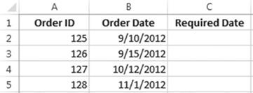
Figure8-51.Datausedforthisexample
The function that follows will be entered in
cell C2 and then copied down through cell C5.
=DATE(YEAR(B2),MONTH(B2)+3,DAY(B2))
Figure 8-52 shows the result. The month in cell B4 is 10. Adding 3 to 10 should give us a month of 13, but
Excel
is smart enough to know there isn�t any month 13 and automatically adjusts
the date so that the month
becomes January. Adding 3 to the month in cell B5 automatically adjusted the month to February.
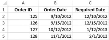
Figure 8-52.Excel
automatically adjusted dates that went past the year
299
CHAPTER 8 ■ EXCEL�S PRE-EXISTING FUNCTIONS
Excel will also automatically adjust
the date if there ends up being more days than there are in a month.
DAYS�Returns the Number of Days Between Two Dates
The DAYS function is used to find the number
of days between
two dates.
The syntax for the DAYS function is
DAYS(end_date,start_date)
Argument descriptions are
end_date and start_date are the two dates between
which you want to know the
number of days.
If the date 1/5/1994 was in cell A1 and you wanted to know how many days were between that date and today�s
date, you would use today�s
date as the end date and 1/5/1994
as the start date. You would enter the
following formula in a cell.
=DAYS(TODAY(),A1)
In this exercise we will use the DAYS function
to determine how many days fall between a series of start and end dates.
1.
Create a new worksheet named �DAYS.�
2.
Enter the data as shown in Figure
8-53:
a.
Enter and format the column
heads.
b.
Enter the date in cell A2 and then hold down the Ctrl key while you use the AutoFill Handle to
copy the date down through
cell A12. Remember
holding down the Ctrl Key copies the cell rather than creating
a series.
c.
Enter the date in cell B2 and drag the
AutoFill Handle from cell B2 to B5.
d.
Enter the date in cell B6 and drag the AutoFill Handle from cell B6 to B10. See Figure
8-53.
300
CHAPTER 8 ■ EXCEL�S PRE-EXISTING FUNCTIONS
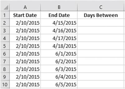
Figure8-53.DateenteredusingAutoFillHandle
3.
In cell C2 enter =DAYS(
4.
Select cell B2 for the end_date argument. Enter a comma
5.
Select cell A2 for the start_date argument. See
Figure 8-54.
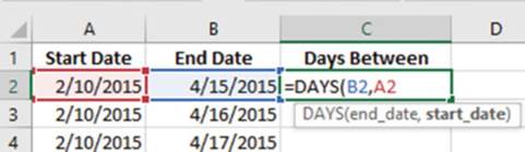
Figure 8-54. Cell A2 selected
6.
Press Ctrl + Enter. Use the AutoFill
Handle to copy the formula
down through cell C10. Figure
8-55 shows the result.
301
CHAPTER 8 ■ EXCEL�S PRE-EXISTING FUNCTIONS
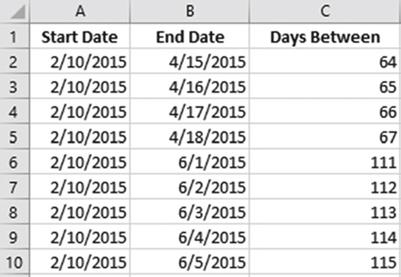
Figure8-55.ResultofusingDAYSfunctionincolumnC
Now that you have experience using the DAYS function try the following exercises:
Find out how many days you have been alive.
1.
In cell A11 enter your birthday.
2.
In cell B11 enter =TODAY()
3.
In cell C11 enter =DAYS(B11,A11)
Find out how many days till Christmas
1.
In cell A12 enter =TODAY()
2.
In cell B12 enter the date for Christmas for the current year
3.
In cell C12 enter the DAYS function to compute
the number of days between the current date and Christmas.
You have learned
how to handle dates and extract just the portion
of a date that you want. Don�t
forget that you can�t
use a date directly in a math formula; rather,
you must use the cell address of the date in the formula.
Summary
This chapter dealt
with functions. You have learned
the two ways of entering
a formula: either
directly into a cell or by using
the Insert Function
option. The Insert
Function dialog box helps you find the function you want
to use. Another
benefit of the Insert Function
dialog box is that it shows the result for each argument that you enter. You might want to use Insert
Function
until you become
very familiar with the function
and
then switch to the quicker
method of entering
functions directly in the cell. You have seen how functions can determine what needs to be done based on if
a condition exists or not.
The next chapter deals with handling errors and protecting
the workbook from someone inadvertently or
purposefully enters something he shouldn�t.
302
CHAPTER
9
Auditing,
Validating, and Protecting Your Data
As the creator of the Excel
workbook, it is your primary responsibility to ensure that the data on the worksheets has been entered
correctly.
You may not have control of the source of the data, but it is your responsibility to ensure that you
enter the data you are given without error. Poor data and incorrect entries can ruin a business. Errors made
in
one location may be propagated to other areas in the workbook. Users may be incorporating the data from
your workbooks into their own projects or they may be using your workbooks to base their decisions on.
Excel provides several tools to help you prevent errors from getting into your workbooks, but it is up to
you to incorporate them.
After
reading and working
through this chapter
you should be able to
�
Identify errors
�
Use data validation to prevent errors
�
Circle invalid data and clear
validation circles
�
Check a formula for an error using the IFERROR function
�
Correct circular references
�
Audit formulas by:
�
Tracing dependents
�
Tracing precedents
�
Using the Watch Window
�
Using the EvaluateFormulafeature
�
Have Excel read back your cell entries
�
Use Spell Checker and Thesaurus
�
Protect worksheets and cells
Validating Your
Data and Preventing Errors
Excel has many tools to
help you prevent errors from being entered into your applications, but it is
still up to you to review all your
entries and to check that the results of your calculations and functions look
credible.
303
CHAPTER 9 ■ AUDITING, VALIDATING, AND PROTECTING YOUR DATA
Data
Validation
One of the most important functions an Excel developer can perform is to make sure that errors do not get
into the spreadsheets. You need to make it as easy as possible
for the user to understand what is to be entered and as easy as possible
to enter the data. You don�t want the user to have to guess
what it is he is
supposed to enter and then
make a wrong assumption. One way to make sure data is entered correctly is by using the
DataValidationfeature. Data validation
consists of various validation rules that specify the criteria for how the data is to be entered. If
the data is still entered incorrectly you can stop the data from being accepted. If the user has entered
something questionable you can provide her with a warning or information message and then let her decide if
the
data should be accepted or not.
Data
being entered can be restricted to the following:
�
values in a drop-down list
�
a whole number within a specified range
�
a decimal number within a specified range
�
a date within a specified time frame
�
a time within a specified time frame
�
a specified length
�
a value based on the content of another cell
�
a value based on a formula
The
Data Validation button
is located on the Ribbon�s
Data tab in the Data Tools group
(Figure 9-1).
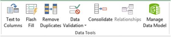
Figure9-1.TheRibbon�sDataToolsgroup
The Data Validation button is divided into two sections. Clicking the upper half of the Data Validation
button brings up the Data Validation dialog box.
The
Data Validation dialog box contains
three tabs (see Figure 9-2):
�
Settings tab: used for setting
the rules for what can be entered
in a cell.
�
Input Message tab: creates a screen tip that tells the user what he should enter in the cell.
�
Error Alert tab: can be used for warning that the entry does not follow the rules you have set up
or it can be used to stop the entry if rules have been broken.
304
CHAPTER 9 ■ AUDITING, VALIDATING, AND PROTECTING YOUR DATA
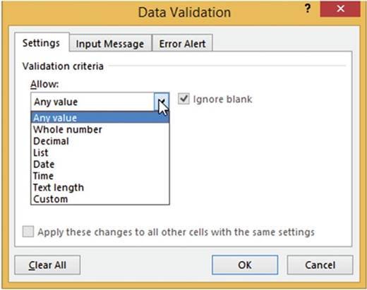
Figure 9-2. Data Validation dialog box
Clicking the lower half of the Data Validation button brings up the three options shown in Figure 9-3.
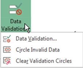
Figure 9-3. Data Validation options
Clicking the first option (Data Validation) gives the same result as clicking the upper half of the button.
305
CHAPTER 9 ■ AUDITING, VALIDATING, AND PROTECTING YOUR DATA
For this exercise you will create data
validation for six fields to warn users about potential problems or to prevent them from making invalid
entries.
All of the entries you will need to make for this practice are in workbook
Chapter 9 on the Validation tab. The worksheet shows what you will need to enter for each option on the
three tabs of the Data Validation dialog box. You can print the worksheet
and then use it as you go through this exercise or you can follow along with the instruction given for each
column.
1.
Open workbook Chapter
9. Click the Val_Entry worksheet
tab. Figure 9-4 shows the column headings from worksheet Val_Entry. The entries that you will need to make
for this exercise
are to the right of the column
headings. There is a second
copy on the Validation worksheet.
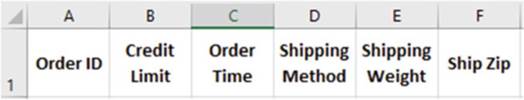
Figure9-4.ColumnheadingsforChapter9workbook
The Order ID must start with either
an SR or a GR. We will prevent the user from entering any other text for the first two characters. We will
perform
a Validation check
for the Order
ID whenever the user enters
a value in any cell in the range A3:A12.
2.
Select the cell range A2:A12.
3.
Click the Data Tab. In the Data Tools group
click the upper
half of the Data Validation button.
The Data Validation window
appears. See Figure 9-5. The workbook Chapter 9 Validation worksheet contains
all of the entries you will be making on the Data Validation window.
4.
Click the Settings
tab if it isn�t already
selected.
5.
Click the down arrow for
Allow and select Custom. The Custom option is for entering
formulas.
6.
Because we want to check the first two characters in the OrderID we will
use the
LEFT function.
The syntax
for the LEFT function is:
= LEFT(text,
[num_chars])
306
CHAPTER 9 ■ AUDITING, VALIDATING, AND PROTECTING YOUR DATA
Arguments are
text is either text or a cell address
containing the text
num_chars is the number of characters you want from the beginning of the string.
Enter the formula =OR(LEFT(A2,2) = "SR",LEFT(A2,2) =
"GR") in the Formula box.
The formula uses the OR function. The formula
tests if the first two characters entered
in cell A2 are SR or GR, then the result is True; otherwise it returns a False. If either argument
is true, then the result
is true and Excel will accept it. We are using cell A3, which
is the first cell in the range.
Excel will automatically adjust the formula
for each cell in the range.
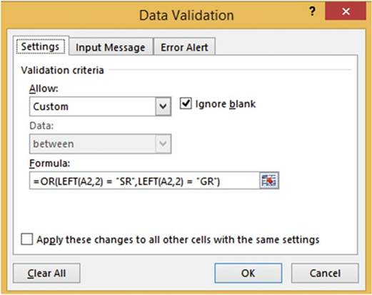
Figure9-5.FormulaensuresthatOrderIDstartswithanSRorGR
7.
Click
the Input Message tab. The entries you need to make
for these exerercises are located to the right of the column headings on the Val_Entry worksheet. You can
see that on the Input Message tab you need to enter a Title of �Order ID Restrictions� and an Input message
of �Order ID�s must start with the letters SR or GR.� Make those entries now. Your Input Message tab should
look like Figure 9-6.
307
CHAPTER 9 ■ AUDITING, VALIDATING, AND PROTECTING YOUR DATA
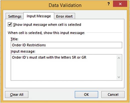
Figure 9-6.Message appears when an Order ID cell is selected
The input message
on the Input Message tab informs the user about any entry restrictions, but if the user breaks the rule
entered on the Settings
tab we want to display
an error message.
8.
Click the Error Alert tab.
9.
Select Stop for the style.
The style of Stop prevents an
invalid entry from being accepted.
10.
Enter the title �Order ID
Error�
11.
Enter the error message
�Order IDs can only start with the letters SR or GR.� See Figure
9-7.
12.
Click the OK button.
308
CHAPTER 9 ■ AUDITING, VALIDATING, AND PROTECTING YOUR DATA
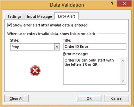
Figure9-7.Createerrormessageformakinganinvalidentry
13.
Click inside cell A2. You should see the message
you created on the Input Message tab (Figure 9-8).
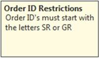
Figure 9-8.Message informing you what needs to be entered
in the cell
14.
Enter KY14 in the cell and then press the Tab key. You should see the error message you
created on the Error
Alert tab. See Figure 9-9.
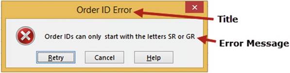
Figure9-9.Errormessageifusermakesinvalidentry
309
CHAPTER 9 ■ AUDITING, VALIDATING, AND PROTECTING YOUR DATA
15.
Click the Retry
button. Enter SR14 in the cell.
Press the Tab key.
Creating
an Error Alert Using No Style
For this Validation we will create a message
informing the user of what the entry should normally
be, but we will not show an Error Alert
message or stop the user from making an entry that doesn�t
meet the entry suggestion of entering a value of less than 30000.
1.
Select the cell range B2:B12.
Click the Data Tab. In the Data Tools group click the upper half of the Data Validation button. Click the
Settings tab.
2.
Enter the data in Table 9-1 for the three tabs.
Table9-1.EntertheDatainThisTablefortheThreeTabs

Tab������� Option���� Value Selected or Entered
Settings
Input Message
Error
Alert
Allow��� Whole number
Data���
less than
Maximum�
30000
Title��� Credit Limit Restrictions
Message��
Credit limits
are usually less than 30000
Remove the check mark from the �Show error alert after invalid data is entered�
check box.

Removing the check mark from the �Show
error alert after
invalid data is entered� (Figure
9-10) prevents any other entries
from being made on this tab. Making
this change allows
the user to enter a value that breaks the rule set on the Settings tab. The Input
Message will display
but there will be no Error Alert
message.
3.
Click the OK button.
310
CHAPTER 9 ■ AUDITING, VALIDATING, AND PROTECTING YOUR DATA
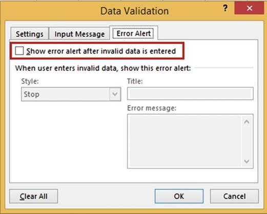
Figure 9-10.Remove the check mark from �Show
error alert after
inalid data is entered�
4.
Double-click cell B2. The input
message displays.
5.
Enter 90000 and press Tab. The
entry is accepted and no error message
appears.
Creating a
Warning Style and Using a Time Restriction
For this Validation you will create
a Warning for the Order
Time column for entries that are not between 8:00 AM and 5:00 PM.
1.
Select the cell range C2:C12.
Click the upper
half of the Data Validation button. Click the Settings tab.
2.
Enter the data in Table 9-2.
311
CHAPTER 9 ■ AUDITING, VALIDATING, AND PROTECTING YOUR DATA
Table9-2.EntertheDatainThisTable

Tab�������� Option������ Value Selected or Entered
Settings
Input Message
Error
Alert
Allow����� Time
Data����� between
Start time��� 8:00 AM
End time��� 5:00 PM
Title���� Order Time
Restrictions
Message���
The time entered should be between 8 AM and 5:00 PM
Style����� Warning
Title���� Possible Error
Message���� The time should
be between 8:00 AM and 5:00 PM unless there
is a specific reason for this.
3.
The Warning style warns you that an error may have been made and lets you decide
if you want to accept the entry or not. Click the OK button.
4.
Enter 6:00 PM in cell C2 and then
press the Tab
key. The error message in
Figure 9-11 appears.
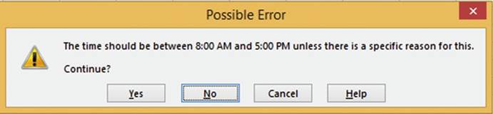
Figure 9-11.Warning message that appears
if an invalid time was entered
If you click the No button, Excel selects the cell for editing and you can make a change. If you click the
Yes button, the entry you made will be accepted.
5.
Click the No button, then
change the entry to 1:00 PM, and
then press the Tab key.
Creating
a List Restriction
This Validation limits the entries for the
Shipping Method column to those of a list that we create.
1.
Select the cell range D2:D12.
Click the Upper
half of the Data Validation button. Click the Settings Tab.
2.
Enter the data in Table 9-3.
312
CHAPTER 9 ■ AUDITING, VALIDATING, AND PROTECTING YOUR DATA
Table9-3.EntertheDatainThisTable

Tab������� Option����� Value
Selected or Entered
Settings
Input Message
Error
Alert
Allow���� List
Source��� Freightways, FED EX, Parcel Post, UPS
Title���� Shipping Method
Restrictions
Message���
You can only select a Shipping Method from the list.
Style���� Stop
Title���� Shipping Method
Error
Message���
You can only pick a Shipping Method from the list.

Figure 9-12 shows how the Settings tab should look.
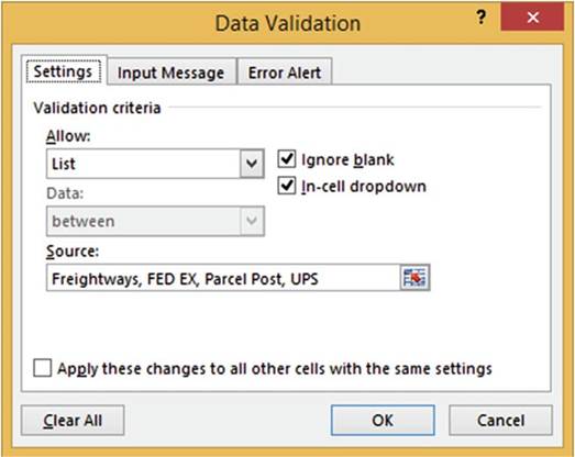
Figure9-12.TheSettingsafterenteringthedatainTable9-3
3.
Click the OK button.
4.
Double-click inside cell D2.Click the down arrow to the
right of the cell. A list box appears from which you can select one of
the entries you created (Figure 9-13).
313
CHAPTER 9 ■ AUDITING, VALIDATING, AND PROTECTING YOUR DATA
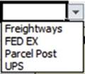
Figure9-13.Listboxfromwhichtoselectanentry
If you type something else into the cell that
is not in the list you will get the message shown in Figure 9-14.
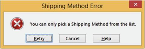
Figure 9-14.Error
message if you enter something
that is not in the shipping list
5.
Click the down arrow in cell D2 and select UPS from the list. Press the Tab key.
Creating
an Information Style Error Alert
This Validation for the Shipping
Weight column displays
a warning message
if someone tries
to make an entry greater
than 35.
1.
Select the cell range E2:E12.
Click the upper
half of the Data Validation button. Click the Settings Tab.
2.
Enter the data in Table 9-4.
314
CHAPTER 9 ■ AUDITING, VALIDATING, AND PROTECTING YOUR DATA
Table 9-4. Enter This Data

Tab������� Option����� Value
Selected or Entered
Settings
Input Message
Allow��� Whole number
Data���� less than
or equal to
Maximum�� 35
Title���� Shipping Weight
Information
Message��� Orders Weighing more than 35 lbs. are usually shipped
using Freightways.
Error
Alert�� Style����� Information
Title���� Shipping Weight
Information
Message��� The weight on this Order is more than 35 lbs. Did you ship it using Freightways????
The Information style will not prevent
someone from entering a value that does not
meet the criteria set on the Settings tab.
3.
Click the OK button.
4.
Double-click cell E2. Enter 45 and then press tab. A Warning
message appears (Figure
9-15).
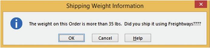
Figure9-15.Information-stylemessage
5.
Click the OK button. The cursor
moves to cell F3.
Creating a Custom
Restriction That Restricts the Number of Characters That �Can
Be Entered
This Validation restricts the
Zip Code column to either 5 or 9 characters.
1.
Select the cell range F2:F12.
Click the upper half of the Data Validation button. Click the Settings
tab.
2.
Enter the data in Table 9-5.
315
CHAPTER 9 ■ AUDITING, VALIDATING, AND PROTECTING YOUR DATA
Table 9-5. Enter This Data

Tab������� Option���� Value Selected or Entered
Settings
Input Message
Error
Alert
Allow��� Custom
Formula�� =OR(LEN(F2)=5, LEN(F2) =9)
Title��� Zip Code
Restrictions
Message�� Please enter a 5 or 9 digit zip
code.
Style��� Stop
Title��� Zip
Code Error
Message��
You can only enter 5 or 9 digits for the zip code.

An OR function tests if any of the arguments are
true; if one is true then the result is true and Excel will accept it. Excel will automatically adjust the
formula for each cell in the range.
3.
Click the OK button.
4.
Double-click inside cell F2. Enter
3845 then press
the Tab key. The message
in Figure 9-16 displays.
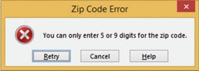
Figure 9-16. Error message
5.
Click the Retry button. Change the zip code to 38451 and then press the Tab
key.
6.
Click inside cell A3. Type the rest of the data as shown in Figure 9-17. Cells C3 and C4 will give
a time warning.
Click the Yes button for both of them. Cells E2 and E4 will give a weight warning.
Click the OK button for both of them.
316
CHAPTER 9 ■ AUDITING, VALIDATING, AND PROTECTING YOUR DATA
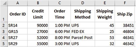
Figure 9-17. Enter this data
Circling
Invalid Data
We set the Credit Limit, Order Time, and Shipping Weight to use the Warning and Information
styles rather than the Stop Style on the Error Alert tab. This allowed us to break the rule that
we had set up on the Settings tab. We can have Excel place a circle around all those cells
that broke a rule.
1.
Click the Validation
button drop-down arrow then select Circle Invalid Data. See Figure 9-18.
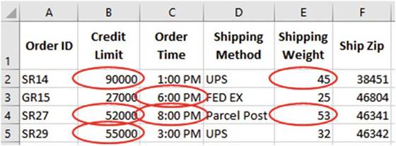
Figure9-18.Cellsthatbrokearulearecircled
2.
Click the Validation
button drop-down arrow and then select Clear
Validation Circles.
Expanding the
Size of the Validation area
We have set
the Validation to work on rows 2
through 12. Now let�s extend it
through row 20.
1.
Click inside cell D12. There is
a drop-down arrow to the right of it.
2.
Click inside cell D13. There is
no drop-down arrow to the right of it.
What if we later need to add data beyond
row 12? We can extend
the Validation area by using
Paste Special.
3.
Select the cell range A2:F2. Press Ctrl + C to copy the cells.
317
CHAPTER 9 ■ AUDITING, VALIDATING, AND PROTECTING YOUR DATA
■
NoteYou can actually use any of the cells that contain the Validation you want to use when
performing the copy.
4.
Select the cell range A13 to F20.
5.
On the Home tab in the Clipboard group
click the Paste button down arrow. Select Paste Special. Select Validation. See Figure 9-19. Click the OK
button.
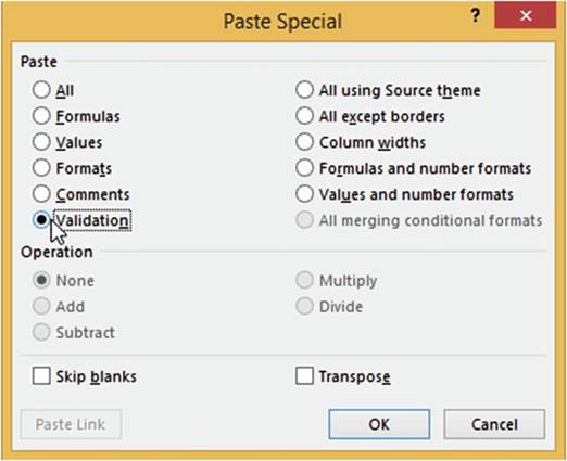
Figure9-19.SelectValidationfromthePasteSpecialwindow
The Validation Range has now been extended to row 20.
6.
Enter the following data in row 13. See Figure 9-20.

Figure9-20.Enterthisdatainrow13
You have
learned how to use data validation to prevent users from making data entries
that you didn�t intend
for them to make. Next, you will see that when Excel comes across an entry it
can�t understand, it displays an error code.
318
Evaluating
Formulas
CHAPTER 9 ■ AUDITING, VALIDATING, AND PROTECTING YOUR DATA
Excel can often recognize
when there is a problem
with a function, such as informing you when there are circular references. Table 9-6 shows some of the
errors that Excel displays when it finds what it thinks is an error.
Table9-6.ErrorValueMessages

Error
Value�
Meaning����������������� Causes
#DIV/0� Division by zero�������� Error occurs
when attempting to divide a value by zero or if you
try to divide
a value by an empty
cell.
#N/A�� No value available������� This isn�t necessarily an error. It means that what you are looking for
doesn�t exist in your lookup table. For example, if you use VLOOKUP and there was no match for your
lookup_value argument.
#NAME?� The formula contains unrecognized text� Error occurs when you use a nonexistent range
name or sheet name, or the function name is misspelled, or you forget to put quotation marks around a text
string in a formula.
#NULL!� Cell references are not separated correctly Error occurs if you use a space instead of a
comma to separate cell references or ranges. The error can also occur
if you forget to put an operator
between cell references, such
as forgetting to put one of the plus signs in a
formula such as = B3 + C3 D3
#NUM!�� Formula uses an invalid number��� The formula is using an invalid number such as
entering an invalid serial date number
#REF!�� Invalid cell reference������� Error occurs when the formula uses a cell reference that for some
reason no longer exists, such as if you deleted a value that was referenced by a formula.
#VALUE!� Formula used the wrong type of data for an argument
Used text for an argument that was used for a mathematical operation.
Using IFERROR
The IFERROR function checks a formula (or expression) and returns the results if there is no error; otherwise
it returns a value you specify.
The syntax for the IFERROR function is:
=IFERROR(value,
value_if_error)
Arguments:
value is the expression being tested.
value_if_error is the text that will be returned
if there is an error
in the expression
319
CHAPTER 9 ■ AUDITING, VALIDATING, AND PROTECTING YOUR DATA
The IFERROR can�t distinguish the type of error. The error could be DIV/0, #NAME, #N/A, #REF, and so on. What
is used as the value_if error argument will be displayed regardless of the error type.
The formula
=IF(Sales
> 25000,B3 + B2, B4 + B2) would return a #NAME? error if the Sales range
didn�t exist. If you wanted to test for such a condition, you would use the formula
=IFERROR(IF(Sales >
25000,B3 + B2, B4 + B2),"Range name doesn't exist")
If the Sales range didn�t exist, Excel would display Range name doesn�t
exist in the cell where you entered the formula. If the range did exist, the IF function would
perform as normal.
In Figure 9-21, cell C1 contains the formula =a1/b1 and cell C2 contains the formula =a2/b2. Cell C1 has a
divide by zero error. Cell C2 has a #VALUE! error because it attempted to divide by an alpha character.
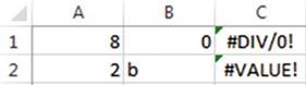
Figure9-21.Invalidvaluesforformulas
You could
make these messages
more meaningful by using the IFERROR function. Entering
the formula
=IFERROR(A1/B1,"Divided by Zero") into cell C1
and the formula =IFERROR(A2/B2,"Divided
by
text")
in cell C2 would produce the result shown in Figure 9-22.
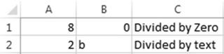
Figure9-22.MeaaningfulmessagescreatedfromIFERRORfunction
■
NoteBe careful
how you use the IFERROR function. If we used the formula =IFERROR(A1/B1,"Divided by Zero") in both
cell C1 and C2 the result would be the same; both would display
�Divided by Zero.�
Correcting
Circular References
A circular reference occurs when a formula in a cell refers to itself either directly or indirectly. This is
usually
something you do not want to occur; however, there are rare occasions when you do (e.g., when doing
iterative calculations).
Figure 9-23 shows
a circular reference. The cell address
A4 is used in a formula in cell A4.
320
CHAPTER 9 ■ AUDITING, VALIDATING, AND PROTECTING YOUR DATA
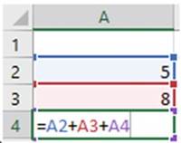
Figure 9-23.The
formula in cell A4 references its own cell address
The first time you create a circular reference on a worksheet you will see the message in Figure 9-24.
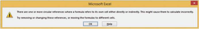
Figure9-24.Messageforfirstcircularreference
When you click the OK button Excel places a zero in the cell that contains the circular reference. See Figure
9-25. You will have to evaluate the formula to determine what it should be.
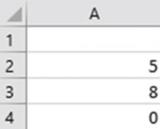
Figure 9-25.Excel
places a zero in a cell that contains the circular reference
It is easy to
accidentally create a circular reference when you are using the SUM function and you drag across the
cells that are to be summed and you include the formula cell. See Figure 9-26.
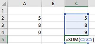
Figure9-26.TheSUMfunctionincludesitsownaddressinitsargument
321
CHAPTER 9 ■ AUDITING, VALIDATING, AND PROTECTING YOUR DATA
Figure 9-27 shows an indirect circular reference. The formula
in cell A2 includes the address C2, which in turn uses cell A2 in
its address.
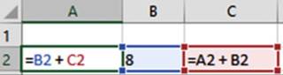
Figure9-27.Indirectcircularreference
After you have entered an indirect circular reference, Excel displays tracer arrows to show you which cells
are involved in the circular reference. See Figure 9-28.
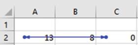
Figure 9-28.Tracer
arrows show which cells are involved in the circular
reference
Double-clicking the arrow in cell A2 makes C2 the active
cell. Double-click it again and cell A2 becomes the active cell again.
Formula Auditing
The Excel Formula Auditing
group has tools for tracking the relationship between cells and the formulas they use.
The Formula Auditing group is located on the Ribbon�s Formulas tab. See Figure 9-29.
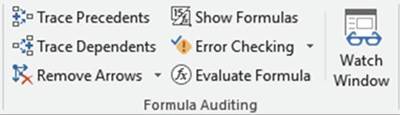
Figure 9-29. Formula Auditing tools
Tracing
Precedents and Dependents
Precedents are values from
other cells that are used in a formula. Dependents are values that are affected
by a formula. Tracing
precedents and dependents gives you a visual view of the relationship between
cell values and formulas. A value can
be both a precedent and a dependent. Select the cell that contains the formula you want to check and then
click the
Trace Precedents button. Clicking a formula and then clicking the precedents button will show all of the
cells whose values are used in the formula.
322
CHAPTER 9 ■ AUDITING, VALIDATING, AND PROTECTING YOUR DATA
Figure 9-30 shows the precedents for
cell A5 and C5. Since individual cells were used in the cell A5 formula, it shows a dot for each
precedent. A cell range was used in the C5 formula, so it shows a dot for the first precedent and a line
representing the others.
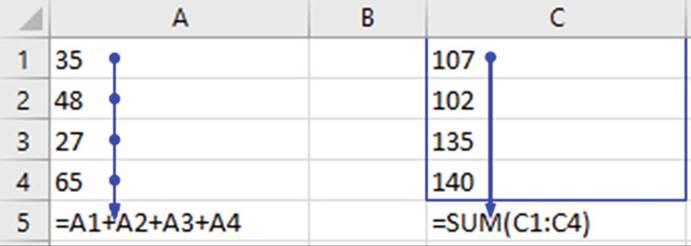
Figure9-30.PrecedentsforcellA5andC5
This exercise will take you through tracking
what formulas the selected cell was used in (dependents) and finding which
cells feed into it (precedents). You will also remove the precedent and dependent arrows.
1.
Open workbook Chapter
9.
2.
Click the tab for the Precedent worksheet.
Figure 9-31 shows the
formulas used in the worksheet.
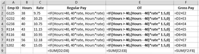
Figure9-31.Formulasusedinworksheet
Creating
Dependent Tracer Lines
1.
Click cell B2. Click Trace
Dependents. The Tracer
lines show that cell B2 is used in the formulas in cell D2 and E2.
323
CHAPTER 9 ■ AUDITING, VALIDATING, AND PROTECTING YOUR DATA
2.
Click cell C3. Click Trace
Dependents. The Tracer
lines show that cell C3 is used in the formulas in cell D3 and E3.
3.
Click inside cell D4. Click Trace Dependents. The Tracer lines
show that cell D4 is used in the formulas
in cell D9 and F4.
4.
Click inside cell E5. Click Trace Dependents. The Tracer lines show that cell E5 is used in the
formulas in cell E9 and F5.
5.
Click inside cell F5. Click Trace Dependents. The Tracer lines show that cell F5 is used in the
formula in cell F9. Figure 9-32 shows all the Dependent lines you have created.
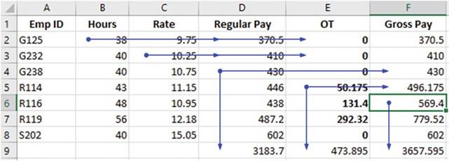
Figure 9-32. Dependent lines
Removing
Dependent Tracer Lines
1.
Click the Remove Arrows down arrow. Click Remove Dependent Arrows. See Figure
9-33.
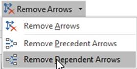
Figure9-33.SelectRemoveDependentArrows
This removes the Dependent Tracer
line from the selected Cell.
2.
Click the Remove Arrows down arrow. Click Remove Arrows.
This removes all the Tracer
lines.
324
CHAPTER 9 ■ AUDITING, VALIDATING, AND PROTECTING YOUR DATA
Creating
Trace Precedent Lines
1.
Click cell D2. Click Trace
Precedents. The Precedent lines show the cells that feed into the formula
in cell D2.
2.
Click cell D9. Click Trace
Precedents. The Precedent lines show the cells that feed into the formula
in cell D9.
3.
Click cell F9. Click Trace
Precedents. The Precedent
lines show the cells that feed into the formula
in cell F9.
4.
Click the Remove
Arrows down arrow.
Click Remove Arrows.
All arrows should now be
removed.
You have
learned how to create tracer lines that show where the values used in your
formulas are
coming from
and what cells are using the results of those formulas. Next, you will learn to
add the cell
addresses of
those cells you want to closely monitor to a Watch Window. The Watch Window
will reflect any changes
in the values of these cells.
Using the Watch Window
The Watch window is useful when you want to see how the values you are entering
are affecting the results of formulas that you can�t
see. The formula
may not be visible because
it is on another worksheet. The formula may also be on the same worksheet, but it is in a location where
you would have to repeatedly scroll back and forth.
The Watch Window button is located on the Formulas
tab in the Formula Auditing
group. See Figure
9-34.
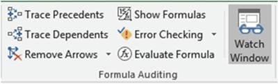
Figure9-34.TheRibbon�sFormulaAuditinggroup
Cells are added to the Watch Window by clicking the Watch Window button, selecting the cells to be added, and
then clicking the Add Watch button. Cells are removed from the Watch Window by selecting the items you want
to remove and then clicking the Delete Watch button.
In this exercise, you will add
cells to the Watch Window and then remove cells.
1.
Open Workbook Chapter 9. The workbook contains
worksheets for January, February, and March Sales and a worksheet that Totals those sales as
well as providing the January Sales total amounts for salesmen 127 and 235.
2.
Click the Sales-Totals worksheet.
325
CHAPTER 9 ■ AUDITING, VALIDATING, AND PROTECTING YOUR DATA
Adding
Cells to the Watch Window
1.
Click the Ribbon�s
Data tab. In the Formula
Auditing Group click the Watch
Window button.
2.
Hold down the Ctrl key while selecting cells B1, B4, B6, and B8.
3.
Click the Add Watch button. See Figure 9-35.
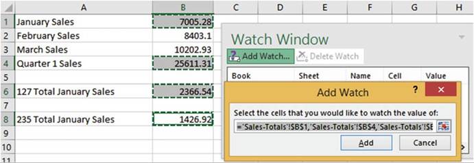
Figure9-35.ClicktheAddWatchwindow
The Watch Window
displays values for the cells you selected
as well as their formulas.
Click the Add button on the Add Watch dialog
box.
4.
Click the Jan-Sales worksheet tab. See Figure 9-36. Change
the value in cell C3 to 600.00.
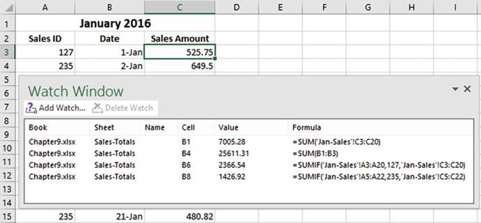
Figure9-36.ChangevalueincellC3to600.00
326
CHAPTER 9 ■ AUDITING, VALIDATING, AND PROTECTING YOUR DATA
You can see how changing the
value in cell C3 to 600 has changed the values in cells B1,
B4, and B6 on the Sales-Totals worksheet. See Figure 9-37. These cells contained the formulas for January
total sales, the quarterly sales, and salesman
127.
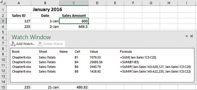
Figure 9-37. Watch Window
5.
Change the value
in cell C4 to 700. It
changed the values for the January totals,
quarterly totals, and totals for salesman 235.
Removing
Cells from the Watch Window
Remove the cells from the Watch Window by clicking the items and then
clicking the Delete Watch button.
You have learned how to control what cells are monitored by either adding or removing cell addresses
from the Watch Window. Next, you will learn how to evaluate a nested function, step by step. Nested
functions can be very complex and it becomes difficult to determine the different parts. The Evaluate
feature goes through the parts of the nested function one step at a time while it shows intermediate
results.
Using the Evaluate Formula Feature to Evaluate a Nested Function One Step at a Time
The
Evaluate Formula feature
helps you see step by step how a nested
function works.
In this exercise, you evaluate a nested formula.
1.
Open workbook Chapter
9.
327
CHAPTER 9 ■ AUDITING, VALIDATING, AND PROTECTING YOUR DATA
2.
Click the Evaluate
worksheet tab.
Cell B2 has a range name of Sex. Cell C2 has
a range name of Age. The formula in cell D2 test
if Sex has a value of F
or Age has a value of 21
or greater.
If either
condition is True, it will display a B; otherwise
it will display a blank.
See Figure 9-38.
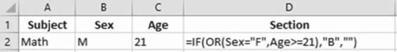
Figure 9-38. Nested formula
3.
Click inside cell D2.
4.
Click the Ribbon�s
Formulas tab. In the Formula
Auditing group click Evaluate Formula
to open the Evaluate Formula
dialog box shown in Figure 9-39.
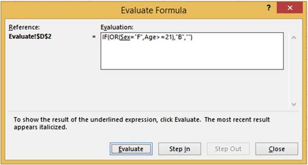
Figure 9-39. Evaluate Formula window
5.
Click the Step In button.
The Step In button displays
what cell is associated with the range name Sex. See Figure
9-40.
328
CHAPTER 9 ■ AUDITING, VALIDATING, AND PROTECTING YOUR DATA
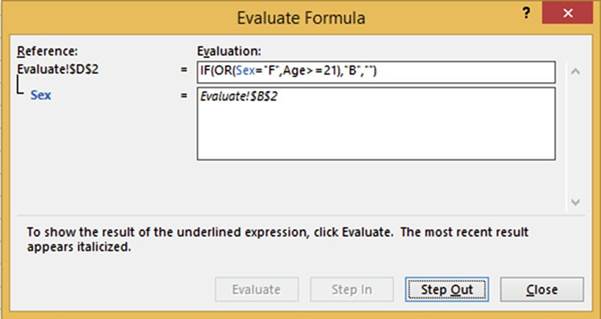
Figure 9-40. Using Step In
6.
Click the Step Out button.
The Evaluate Formula
dialog box shows that there is an M in cell B2. It compares
to see if it is equal to F. See Figure 9-41.
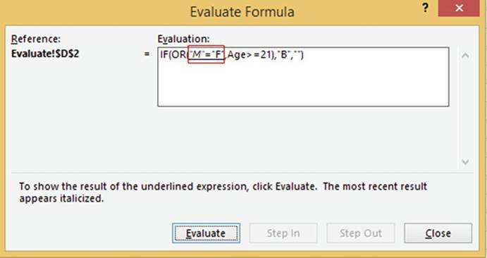
Figure 9-41. Using Step Out
7.
Click the Evaluate
button. M is not equal to F so the expression displays
a FALSE as in Figure 9-42.
329
CHAPTER 9 ■ AUDITING, VALIDATING, AND PROTECTING YOUR DATA
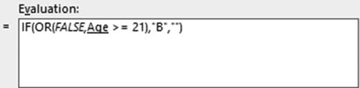
Figure9-42.M=FisevaluatedtoFALSE
8.
Click the Step In button.
You can see in Figure
9-43 that cell C2 has a range
name of Age.
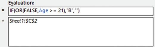
Figure9-43.CellC2hasarangenameofAge
9.
Click Step Out. The Evaluation Formula window shows
that we have a value
of 21 in cell C2. It compares
to see if it is greater than or equal
to 21. See Figure 9-44.
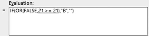
Figure9-44.TheAgerangehasavalueof21
10.
Click the Evaluate button. The condition 21>=21 evaluates to TRUE. See Figure 9-45.
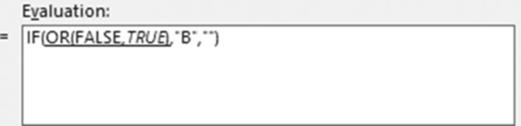
Figure9-45.Thesecondcondition21>=21evaluatestoTrue
330
CHAPTER 9 ■ AUDITING, VALIDATING, AND PROTECTING YOUR DATA
11.
Click the Evaluate
button. The OR function returns a TRUE if either condition is true. The second condition was True so the
function
returns a TRUE. See Figure 9-46.
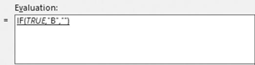
Figure9-46.TheresultoftheORfunctionisTRUE
12.
Click the Evaluate
button. The formula
evaluates to TRUE so it displays the true_ value which in this case is B. Close the dialog box.
Proofreading Cell Values�Have Excel Read Back Your Entries
Excel can help you
proofread your spreadsheet by speaking the values entered in the cells. You can
verify that you have made the
correct entries by listening to the Excel speaker while you look at the paper
from which you made the entries.
This
option is not included on the Ribbon;
it needs to be added there or to the Quick Access Toolbar.
Instead of adding the Proofreading options to the Ribbon, we will add them to the Quick
Access Toolbar.
1.
Right-click the Quick Access Toolbar and select Show Quick Access Toolbar Below the Ribbon.
2.
Right-click the Quick Access Toolbar
and select Customize Quick Access Toolbar,
3.
In the Choose
commands from drop-down box select Commands Not in the Ribbon.
4.
Scroll down using the scroll
bar until you come to Speak Cells.
Click Speak Cells and then click the Add button.
Do the same thing for the next four options.
See Figure 9-47.
331
CHAPTER 9 ■ AUDITING, VALIDATING, AND PROTECTING YOUR DATA
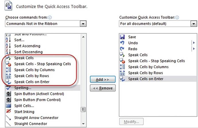
Figure9-47.AddSpeakcommandstotheQuickAccessToolbar
5.
Click the OK button. You should now have five
new buttons on your Quick Access Toolbar. See Figure 9-48.

Figure9-48.SpeakcommandsplacedontheQuickAccessToolbar
6.
Click the Speak
Cells on Enter button on the Quick Access Toolbar. You will get a voice confirmation that anything
that you enter
into the cells will be read back to you.
7.
Enter the data in Figure 9-49 into
a new spreadsheet. As you enter the
data, the information will be read
back to you.
332
CHAPTER 9 ■ AUDITING, VALIDATING, AND PROTECTING YOUR DATA
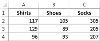
Figure 9-49. Enter this data
8.
Click Speak Cells on Enter again. This turns off the Speak as you Enter option.
9.
Select cells A1:C4. Click the Speak Cells by Rows
button on the Quick Access Toolbar. Click the Speak
Cells button on the Quick
Access Toolbar. Excel speaks the data
in row
order.
10.
Click the SpeakCellsbyColumnsbutton.
Click
the Speak Cells button. Excel speaks the data in column order.
Click
the Speak Cells�Stop Speaking Cells button before Excel has finished reading all of the data. Excel
provides the capability to stop speaking at any point and then continue from that point.
Now if you click Speak Cells, Excel will start reading from the point where you clicked the Speak
Cells�Stop Speaking Cells button.
Spell Checking
The Spelling and Thesaurus buttons are located on the Review tab, in the Proofing group. See Figure 9-50.
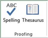
Figure 9-50. The Proofing group
To avoid the
embarrassment of turning in a workbook with misspelled words you should always
check it with Excel�s Spell Checker.
You could test a range of cells or the entire worksheet. If you select a range
of cells before clicking the Spell
Checker, only that range of cells
will be checked. If you have only one cell selected�
or if
you click the Select All button to the left of column A, then it will check the
entire worksheet.
If Excel can�t
find a word in its dictionary, it will display it in the Not in Dictionary text
box. It provides one or
more suggestions of how it thinks it should be spelled in the Suggestions: list
box. See Figure 9-51.
333
CHAPTER 9 ■ AUDITING, VALIDATING, AND PROTECTING YOUR DATA
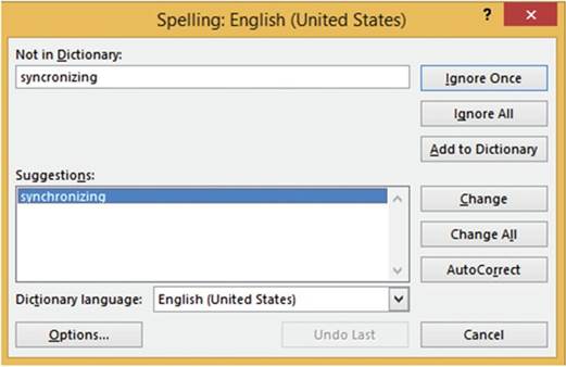
Figure 9-51. Spell Checker
The
purpose of the buttons are as follows:
�
Ignore Once�Tells Excel that you don�t
want to change the spelling
at the current cell but you still want to test the word in other locations.
�
Ignore All�Tells Excel you don�t want to change the spelling
of the word in the Not in Dictionary text box in this location
or in any other location
on the worksheet.
�
Add to Dictionary�Adds the word to Excel�s
dictionary. Excel will never tell you
again that the word is misspelled.
�
Change�Replaces the word in your worksheet cell with the word you have selected in the
Suggestions: list box.
�
Change All�Changes all occurrences in your worksheet of the word in the Not in Dictionary
text box with the one you have selected in the Suggestions: list box.
�
AutoCorrect�Adds the word selected in the Suggestions: list box as the replacement for the
word in the Not in Dictionary for Excel�s AutoCorrect feature.
�
Dictionary
Language�Allows
you to select from one of many different dictionaries.
Thesaurus
If you are looking for a
word that has a similar meaning to a word in your spreadsheet you can use
Excel�s Thesaurus. Just select the word and then click the Thesaurus button.
Figure 9-52
shows that the
word Synchronizingwas
selected when the Thesaurus button was clicked.
334
CHAPTER 9 ■ AUDITING, VALIDATING, AND PROTECTING YOUR DATA
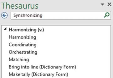
Figure 9-52. Thesaurus
The (v.) next to Harmonizing means that it is a verb. Click a word in the list and it displays similar
meaning words for it.
Figure 9-53 shows that the word Harmonizing was
selected from the list in Figure 9-52 and now words with similar meaning
to Harmonizing are displayed. The (adj.) means
the word is an adjective.
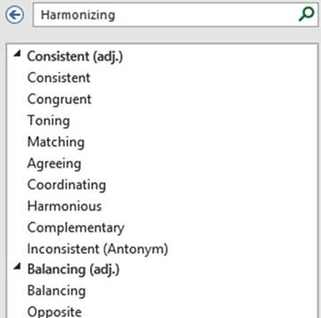
Figure9-53.WordswithsimilarmeaningtoHarmonizing
To
move back in the list of words
click the
 �button.
To replace the
word in your cell with one from the Thesaurus list, right-click the word in the
Thesaurus list and then select Insert. See Figure 9-54.
335
CHAPTER 9 ■ AUDITING, VALIDATING, AND PROTECTING YOUR DATA
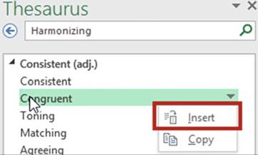
Figure 9-54.Replace a word in your spreadsheet with one from the Thesaurus
list
Protect Worksheets and Cells from
Accidental or Intentional Changes
You can protect your workbook data by preventing users from accidentally or intentionally changing,
adding, or deleting your data.
You can protect your data at the workbook level, the worksheet level or the cell level. You have already seen
how to protect your data on the Workbook level in Chapter 6. You will now see how to use worksheet
and cell level protection.
Protect Your Data at the Worksheet
Level
The commands needed for Worksheet-level and cell-level protection can be found
on the Review tab in the Changes
group. See Figure
9-55.
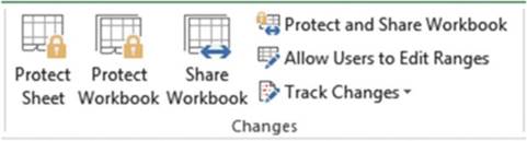
Figure9-55.TheRibbon�sChangesgroup
All cells in a
workbook are locked by default. Locked Cells don�t provide any protection until
you click the Protect Sheet button.
Right-clicking a cell and then selecting Format Cells brings up the Format
Cells window. If you click the
Protection tab you will see that locked is checked. See Figure 9-56.
336
CHAPTER 9 ■ AUDITING, VALIDATING, AND PROTECTING YOUR DATA
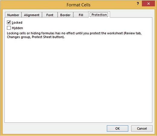
Figure9-56.Cellsarelockedbydefault
In this exercise, you protect a worksheet with a password.
1.
Open workbook Chapter 9. Click the Protect worksheet tab.
2.
Click the Ribbon�s
Review tab. In the Changes
group click the Protect Sheet button. The Protect Sheet dialog box displays. See Figure 9-57.
337
CHAPTER 9 ■ AUDITING, VALIDATING, AND PROTECTING YOUR DATA
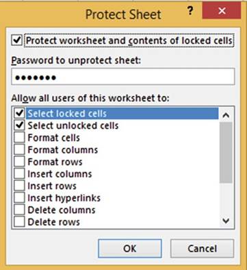
Figure 9-57. Protect Sheet dialog box
The Protect Sheet dialog box lets you assign capabilities to users by checking those options you want to give
them, such as the ability
to format cells or insert rows and columns.
3.
Leave Select locked cells and Select unlocked cells checked.
4.
Enter a password.
■
Caution� Make sure that you remember
the password. You should write
it down somewhere safe. If you forget it, you will not be able to open the worksheet again.
5.
Click the OK button.
6.
Reenter your password to confirm the password you entered
in the Protect Sheet window. See Figure 9-58.
338
CHAPTER 9 ■ AUDITING, VALIDATING, AND PROTECTING YOUR DATA
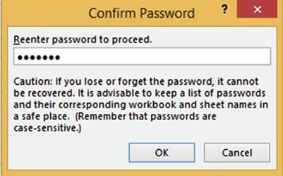
Figure9-58.ConfirmPassworddialogbox
7.
Click the OK button.
8.
Right-click a cell. Notice that Format Cells is dimmed.
9.
Right-Click a row head. Notice
that Insert and Delete are dimmed.
These as well as the other options you didn�t
select in the Protect Sheet window are unavailable.
10.
Try changing a value. You will get the message in Figure 9-59. Click the OK button.
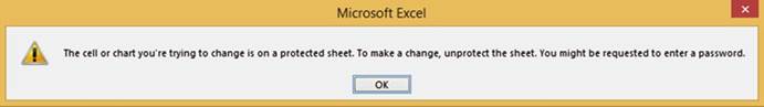
Figure 9-59.Message informing you that what you are trying
to change is protected
11.
Try entering a value in a blank cell. You will get the same message as in Figure 9-59.
12.
In the Changes group, click the Unprotect Sheet.
13.
Enter the same password you entered previously into the Unprotect Sheet dialog box. See Figure
9-60. Click the OK button.
339
CHAPTER 9 ■ AUDITING, VALIDATING, AND PROTECTING YOUR DATA
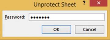
Figure9-60.Enterpasswordtounprotecttheworksheet
The worksheet is now unprotected. You can make any additions or changes to
the data.
Protect Your Data at the Cell Level
You saw
previously where all cells are locked by default. When you click the Project
Workbook button in the Changes
group all those locked cells become protected and you will not be able to enter
any data. Therefore, when
allowing users to make changes to cell data, you don�t protect cells because
they are already protected. Rather, you unprotect those cells that you are willing to let users make
changes to. You need to specify the cells that you are unprotecting before clicking the Protect Workbook
button.
In this practice you will prevent users from
unhiding column F and from making any changes to the formulas or headings.
1.
Open workbook Chapter 9. Click the Protection worksheet tab.
2.
Right-click column head F and then select Hide.
3.
Select cell range A2:C8. Right-click the selected cells and then
select Format Cells.
4.
Click the Protection tab and do the following:
a.
Uncheck Locked. This will unlock
the cell range A2:C8.
b.
Check Hidden. This will prevent
users from unhiding column F.
c.
Click the OK button.
On the Ribbon�s
Review tab, in the Changes
group, click the Protect Sheet button. Enter
a password. Confirm
the password by reentering it.
5.
Try to change a value
in the cell range A2:C8.
You can do so.
6.
Try changing one of the formulas. You will get the message
displayed in Figure 9-61.
340
CHAPTER 9 ■ AUDITING, VALIDATING, AND PROTECTING YOUR DATA
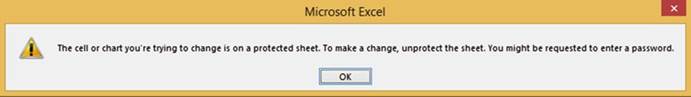
Figure 9-61.Message informing you that what you are trying
to change is protected
7.
Drag across column heads E and G. Right-click the selection; you will see that unhide is dimmed.
8.
In the Changes group click the Unprotect Sheet button.
9.
Enter your password.
Click the OK button. You can now make changes
to all cells.
10.
Drag across column heads E and G. Right-click the selection and then select unhide.
Column F should now be visible.
Summary
Excel has many helpful
features to make sure that data entries are made correctly and, if they aren�t,
to notify you immediately so that you
can correct the error. You have seen how Excel can correct your misspellings and suggest other words to use
from
their Thesaurus. You have seen how you can get visual cues to track
the movement in and out of Formulas. Excel also shows tracer arrows to show which cells are involved in a
Circular Reference.
The next chapter covers how to create, edit, and remove hyperlinks. A
hyperlink is often just called a link. You have most likely used them a lot on the
Internet, linking from one location on the web site to another or to an entirely different
webs ite. Hyperlinks are text or objects that you can click to take you to
somewhere within the current application or applications such as to another workbook, a web site, an e-mail
application, and so on. We will also look how you can combine text from multiple columns along with any
other text you wish to add.
341
CHAPTER 10
Using Hyperlinks, Combining Text, and Working with the
Status Bar
A hyperlink can be either text or an object such as a picture or a chart element that, when clicked,
takes you to another location
(e.g., a specific
location in your document) or brings up information from another file or
web page. You have probably
used hyperlinks on the Internet.
Clicking a hyperlink in a web page can either take you to a different
location on that page or to a completely different web page.
The Concatenation and Flash Fill features allow
you to combine text from multiple cells and add
additional
text.
Also in this chapter
you will learn
how to display information related
to your spreadsheet on the status
bar. After reading
and working through
this chapter you should be able to:
�
Hyperlink to a web page
�
Hyperlink to a file
�
Hyperlink to an e-mail
�
Hyperlink to a location in the current
workbook
�
Create a hyperlink
that will create and open a new workbook
�
Remove hyperlinks
�
Create Concatenation
�
Use Flash Fill
Working with Hyperlinks
Hyperlinks
are usually displayed
in a different color (usually
blue) and often underlined so that they are easily identifiable. To make them even more identifiable, the
mouse cursor changes to a pointing
hand indicator when moved over a hyperlink. You can use hyperlinks in Excel to link to the following:
�
A file or web page (the file could be another spreadsheet file or it could be another type of file
such as a word document)
�
A particular cell in the current workbook
�
A new document
�
An e-mail address
343
CHAPTER 10 ■ USING HYPERLINKS, COMBINING TEXT, AND WORKING WITH THE
STATUS BAR
Hyperlinking to another file opens the file in the program associated with that file type. For example, if
you create a hyperlink to a file with the extension of .docx, Excel will open that file in Word when that
hyperlink is clicked. If you create a hyperlink to a file with the extension of .psd, Excel will open that
file in Photoshop.
To bring
up the Insert Hyperlink Window
you would perform
the following steps:
1.
Click the cell in which you want to place the hyperlink,
2.
On the Ribbon, click
the Insert tab. In the Links group
click the Hyperlink button.
3.
From the Insert
Hyperlink dialog box, do the following:
a.
Select the type of link you wish to create from the Link to pane.
b.
Enter the text
the hyperlink should display in the Text to display text box.
c.
Select or enter the address you want to
hyperlink to and enter any screen tips you want
to display. See Figure 10-1.
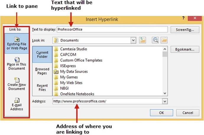
Figure10-1.InsertHyperlinkdialogbox
344
CHAPTER 10 ■ USING HYPERLINKS, COMBINING TEXT, AND WORKING WITH THE
STATUS BAR
The first thing you need to do when creating a hyperlink is to decide what type of link you want to create.
You select the type of link you want to create by clicking the appropriate button in the
Linktopane located on the left-hand side of the window. See Figure 10-1. The options
that appear to the right of the Linktopanechange depending on the button you selected
in the Linktopane. For example, clicking the
ExistingFileorWebPagebutton will display different options to the right
then if you had clicked the Place inThisDocumentbutton.
If there was any text in the spreadsheet cell when you inserted the hyperlink it appears in the Text to
display
text box. Whatever
you enter in this text box will display in your cell; it will override any text currently in the cell. To
the right of the text box is a ScreenTip� button.
Clicking the ScreenTip
button brings up a window in which you can enter a description of the hyperlink. This description will
display for a short time
when the user moves the mouse over the hyperlink. The location of where you are linking
to would be entered in the Address box.
A hyperlink can be removed by right-clicking inside
the cell of the hyperlink and then selecting Remove
Hyperlink from the context menu.
The next four exercises
provide practice in hyperlinking to a web page, to a file, to a location in the
current workbook, and to a newly created
Excel workbook.
In this exercise
you will hyperlink to web pages.
You will use automatic hyperlinking and you will see how to undo automatic hyperlinking. You will also use
words
other than a URL (uniform
resource locator) address
to access a web page.
1.
Create a new workbook named
�Hyperlinks.�
Hyperlinks to web pages are created automatically in Excel if you type an appropriate web address that starts
with http:// or www. in a cell type, provided that you have the option to do this
turned on. You will now check if
that option has been turned on.
2.
Click File ➤ Options.
3.
From the Excel Options dialog
box, select Proofing.
Click the AutoCorrect Options� button on the right
pane of the window.
4.
Click the AutoFormat As You Type tab. Select Internet
and network paths with hyperlinks if it isn�t already selected. See Figure 10-2. Click OK.
345
CHAPTER 10 ■ USING HYPERLINKS, COMBINING TEXT, AND WORKING WITH THE
STATUS BAR
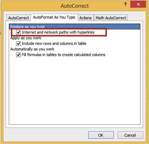
Figure10-2.AutoformatAsYouTypetabintheAutoCorrectdialogbox
5.
Click the OK button on the Excel Options dialog box.
6.
Type www.apress.com in cell A1
then press Enter. Because you set
the option to automatically create hyperlinks whenever you type an appropriate
web address (starts with http:// or www.) a hyperlink is automatically created.
7.
Move your cursor over the text you just entered
in cell A1. The cursor
should display as a pointing
finger. A tooltip
displays the hyperlink address. Click the hyperlink.
8.
Close the Web page.
The hyperlink works, but what if you wanted the words Apress Corporation to appear in the cell instead
of www.apress.com? You will need to edit the hyperlink.
9.
Right-click cell A1 then select Edit
Hyperlink.
10.
Change the text in the Text to display text box
to Apress Corporation. See Figure 10-3. The address should be
correct. Click
OK.
11.
Cell A1 now displays Apress Corporation. Click the text. The Apress web site should
display. Close your Internet browser.
Next, let�s link to an e-mail address.
346
CHAPTER 10 ■ USING HYPERLINKS, COMBINING TEXT, AND WORKING WITH THE
STATUS BAR
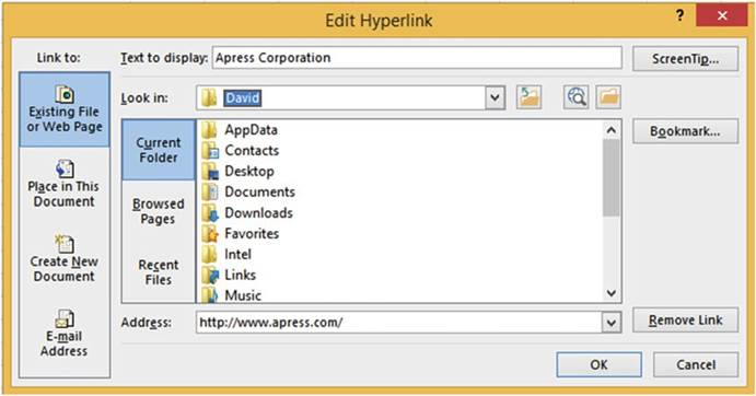
Figure 10-3. Edit Hyperlink dialog box
12.
Type jhall@hotmail.comin cell A3 and then press
Enter.
13.
Click the e-mail address you just created.
When you click a hyperlink to an e-mail
address, your e-mail
program automatically starts
and creates an e-mail message
with the correct
address in the To box, provided
that you have an e-mail
program installed, such as Outlook.
What if you
want to enter a URL that is not hyperlinked?
14.
Type www.MadeinUsa.com in cell A5 and then press
Enter.
15.
Widen the column
so that all the text fits within
the cell. Move your cursor
over the text you just entered in cell A5. The first
w in the hyperlink is underlined. Move your mouse
cursor over the underline and a menu Tag should
appear.
16.
Click the menu tag to bring up a context menu. See Figure 10-4.
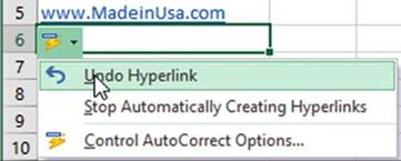
Figure10-4.Contextmenuforhyperlink
347
CHAPTER 10 ■ USING HYPERLINKS, COMBINING TEXT, AND WORKING WITH THE
STATUS BAR
17.
Select Undo Hyperlink. The text remains
but the hyperlink is removed. Now let�s add a hyperlink with a Screen
Tip.
18.
Click cell A7. On the Ribbon, on the Insert tab, in the Links group, click the Hyperlink button.
■
NoteThis
step can also be performed by right-clicking the cell and selecting Hyperlink from the context
menu.
19.
In the Link to pane select
Existing File or Web Page.
20.
Type Professor Office web site in
the Text to display text box.
21.
Type www.professoroffice.com in the Address: box.
Excel automatically adds the prefix
http:// to the address.
22.
Click the Screen Tips� button.
Enter Microsoft Office
and other training
for the ScreenTip text. See Figure
10-5. Press OK.
Click the OK
button for the Insert Hyperlink dialog box.
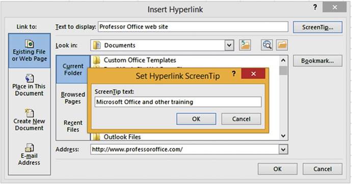
Figure10-5.CreateaScreenTipforthehyperlink
23.
You should now have the hyperlink Professor Office web site in cell A7.
Move your cursor over the hyperlink.
The ScreenTip Microsoft Office and other training displays.
Click
the hyperlink. If you are connected to the Internet this will bring up the ProfessorOffice home page.
Close
the web page.
24.
Right-click cell A7. Select Remove Hyperlink.
348
CHAPTER 10 ■ USING HYPERLINKS, COMBINING TEXT, AND WORKING WITH THE
STATUS BAR
There may be a file that contains more information that you don�t want stored in Excel but you want to have
quick access to. This exercise
shows you how to hyperlink
to a file. When you click that hyperlink the file will open.
1.
Create a new worksheet in your Hyperlinks workbook.
2.
You can use the linkedtext.txt file provided with this book or you can create
your own linkedtext.txt file using the following steps:
a.
Start the Notepad program.
b.
Type the text This
is text that I am linking to. Save
the file with a name of linkedtext. See
Figure 10-6.
Figure 10-6. Create text in Notepad
c.
Save the file to your My Documents folders or a location
you can easily find the path to.
d.
Close the Notepad
program.
3.
Right-click inside cell A5 on your spreadsheet and select Hyperlink�
4.
Enter Notepad file in the Text to display text box. See Figure 10-7.
349
CHAPTER 10 ■ USING HYPERLINKS, COMBINING TEXT, AND WORKING WITH THE
STATUS BAR
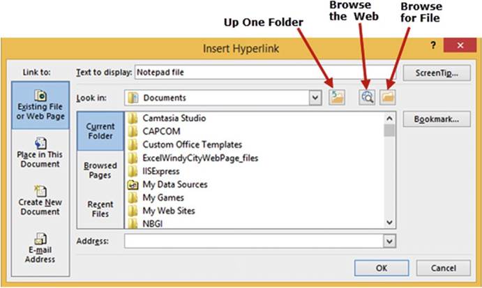
Figure10-7.AddingalinktoafileintheInsertHyperlinkdialogbox
There are several
ways to get the address
(path) and file name in the Address box:
�
You can type the path directly
�
You can click the down arrow to the right of the Look in
drop-down box to get to the correct folder and then select the linkedtext file.
�
You can click the Browse
for File button.
350
CHAPTER 10 ■ USING HYPERLINKS, COMBINING TEXT, AND WORKING WITH THE
STATUS BAR
■
Note� If your file is moved from the path you provide, the hyperlink will not work.
5.
Click the Browse for File button. This brings up the Link to File dialog box in Figure
10-8. Excel thinks you are searching for an Office file, but you are searching for a text file.
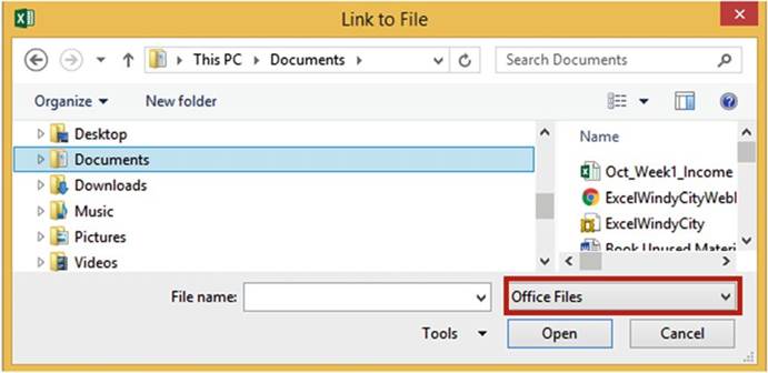
Figure10-8.FindthefileyouwanttolinktointheLinktoFiledialogbox
6.
Click the down
arrow to the right of Office Files and then select All Files. See Figure 10-9. This will enable you
to see
text files.
351
CHAPTER 10 ■ USING HYPERLINKS, COMBINING TEXT, AND WORKING WITH THE
STATUS BAR

Figure 10-9. Select All Files
7.
Find the linkedtext file and then click the Open button.
8.
The address with the linked text file should now appear in the Insert Hyperlink dialog
box. See Figure
10-10. Click the OK button
352
CHAPTER 10 ■ USING HYPERLINKS, COMBINING TEXT, AND WORKING WITH THE
STATUS BAR
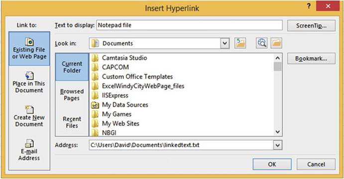
Figure 10-10.The file name with its path is displayed in the Address
field
9.
Click the hyperlink in cell A5. If you get the
message in Figure 10-11, click
the Yes button.
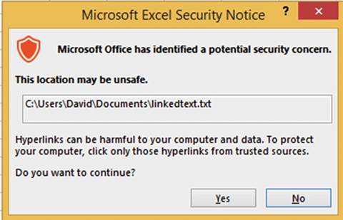
Figure10-11.IgnorethemessageandclicktheYesbutton
The linkedtext.txt file will open either in Notepad or Wordpad,
whichever is your default program for opening text files.
10.
Close the Notepad or Wordpad program.
353
CHAPTER 10 ■ USING HYPERLINKS, COMBINING TEXT, AND WORKING WITH THE
STATUS BAR

The capability to hyperlink to any cell in
your workbook is really convenient when working with a large workbook. In this exercise you will create a
hyperlink that will jump to
cell DA on Sheet2.
1.
Use the same workbook as the previous practice.
2.
Add another worksheet.
3.
On Sheet3, right-click inside cell D7 and select Hyperlink�
4.
Select Place in This Document in
the �Link to� area.
5.
Enter Oct Sales in the Text to display text box.
6.
Enter DA35 for the cell address
in the Type the cell reference text
box.
7.
Select Sheet2 for the Cell
Reference.
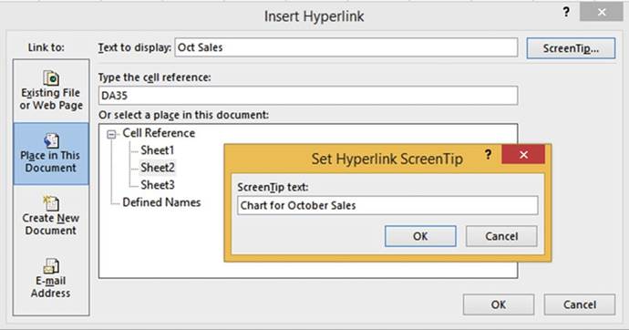
Figure10-12.EnteraScreenTipforthechart
8.
Let�s assume that there is a chart in cell DA35. Click the ScreenTip� button. Enter Chart for
October Sales for the ScreenTip text.
See Figure 10-12. Click the OK button.
9.
Click the OK button in the �Insert Hyperlink� dialog box.
10.
Move your cursor
over the hyperlink. The ScreenTip that you created
displays. Click the hyperlink. The active cell is now DA35 on Sheet2.
354
CHAPTER 10 ■ USING HYPERLINKS, COMBINING TEXT, AND WORKING WITH THE
STATUS BAR
You can create
a hyperlink that,
when clicked for the first
time, creates a new Excel
workbook and then opens that workbook. Every
time you click
it thereafter it will open the workbook. The Excel workbook
will be given
a name that you have assigned within
the Hyperlink options.
1.
Use the same workbook as the previous practice.
2.
On Sheet2 enter the text �Hyperlink to a New Document� in cell A1. Press Ctrl + Enter.
3.
Right-click cell A1 and select Hyperlink.
4.
The Insert Hyperlink window appears. In the Link to: area click Create New Document.
5.
Click the ScreenTip� button.
6.
Enter �Takes you to a newly created
Excel workbook named
Hyperlink_Practice� for the ScreenTip text.
Click OK.
7.
Enter Hyperlink_Practice for the Name of new document.
8.
Change the path if you need to.
In the When to
edit section you have two
options: you can either select to
go immediately
to the
newly created
workbook or create the workbook
and then
open it
whenever you choose to.
9.
Select the option Edit the new
document now. See Figure 10-13.
10.
Click the OK button.
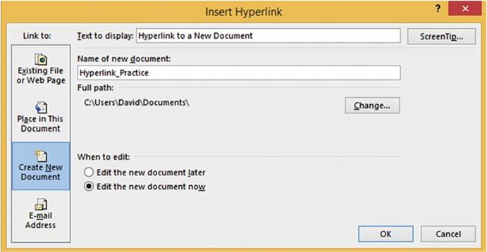
Figure 10-13.Select Edit the new document now on the
Insert Hyperlink window
355
CHAPTER 10 ■ USING HYPERLINKS, COMBINING TEXT, AND WORKING WITH THE
STATUS BAR
11.
Your
cursor should now be in cell A1 of the newly created workbook named Hyperlink_Practice. Go back to your
workbook named Hyperlinks. Click Sheet2 tab cell
A1. Since Hyperlink_Practice has already been created,
Excel
will not try to recreate it,
but it will take you to the Hyperlink_Practice workbook. Before opening the Hyperlink_Practice workbook
Excel may display a Security Notice window. Since you created the hyperlink yourself,
you know it is safe so click the Yes button.
You have learned how to create
and remove hyperlinks. You can create
hyperlinks to open documents
and take you to various
web sites on the Internet, different locations in Excel workbooks, and so on. If you want
a user to get information from another location, then use hyperlinks. It saves the user a lot of time in
locating the information. Next,
you will see how to combine data from different cells (e.g., combining the first, middle, and last names
into one column).
Concatenation and Flash Fill
Joining the data from multiple
cells or joining
cell data with additional text into a single text item is called concatenation. The symbol used to
perform concatenation is the & (ampersand). An ampersand must be
placed between each cell address
and each additional string of text that you�re adding.
For example,
if you wanted to combine
the contents of cell A1 and B1 and place
the results in cell C1 then you would need to place
the following formula
in cell C1 =A1&B1. If you wanted
to place a space between
the data in cell A1 and cell B2 you would need to change
the formula to =A1&" "&B1. A space
between two quotation marks creates a blank
space. If you wanted two spaces between the data you would place two spaces
between the quotation marks.
Figure 10-14 displays
a concatenation starting
in cell A8 that includes
the contents from columns A, B,
and C along with additional text. The formula
entered in cell A8 is
= A2 & "
" & B2 & " used " & "$" & C2 &
" of fuel this week"
The formula was copied down through cell A12 using
the AutoFill Handle.
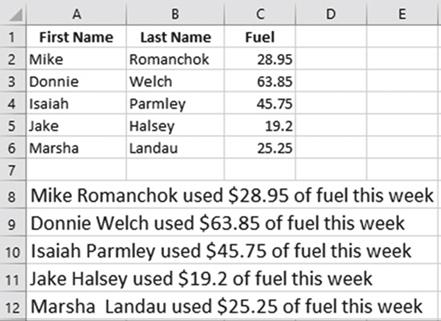
Figure10-14.CombiningdatafromcolumnsA,B,andC
356
CHAPTER 10 ■ USING HYPERLINKS, COMBINING TEXT, AND WORKING WITH THE
STATUS BAR
In this exercise you will use the & character to combine column data
along with other characters.
1.
Open the workbook Chapter 10.
2.
Click the worksheet
Concatenation.
3.
Figure 10-15 shows the data in the worksheet.
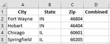
Figure10-15.DatafromConcatenationworksheet
4.
In this exercise you will combine the City, State,
and Zip into a single cell. In
cell D2 enter the following formula
and then press Ctrl + Enter:
=A2 & ",
" & B2 & " "
& C2
The formula displays a comma after the city
followed by a space and provides two spaces between the state and zip.
5.
Widen column D so that the city, state, and zip all fit inside the column.
6.
Drag the AutoFill
Handle from cell D2 down through cell D5. The
result should be as shown in Figure 10-16.
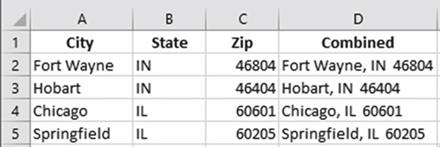
Figure10-16.ResultofusingAutoFillHandle
Now that you have practiced using concatenation, let�s
look at a feature called
Flash Fill, which
can do concatenation without
having to use the &
sign. Flash Fill can speed
up concatenation when you want to
concatenate values that are in a row. You enter
an example of how you want the data to appear. Excel
checks for that pattern
in the other rows and using Flash
Fill copies that pattern down through the column.
357
CHAPTER 10 ■ USING HYPERLINKS, COMBINING TEXT, AND WORKING WITH THE
STATUS BAR
It is still necessary to know how to
concatenate using the & sign when
1.
You are concatenating to a single cell
2.
You are using it
in a formula
3.
What you are concatenating isn�t in the same row
4.
You are using it
in programming code
Let�s look at the same sample that was used for concatenation. Flash Fill would
not have worked
in�
that example because
the concatenation was done on rows that were not in the same row as the data. The Flash Fill does a lot more
than just concatenation. It can be used to find patterns
in your columns
and then to repeat those
patterns in another
column. For example,
you could create
a column that uses the first letter from a column containing middle names or create a column that uses the
day portion
from a date column.
For this example, we will put the concatenation on the same line as the data it is assembling.
In this example you will use Flash Fill to combine multiple columns of
data along with additional text.
1.
Open workbook Chapter 10 if it isn�t already opened.
2.
Click worksheet FlashFill
A.
3.
Figure 10-17 shows the data in the worksheet.
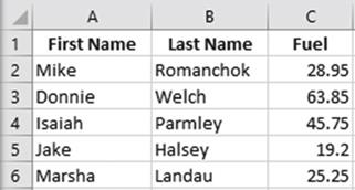
Figure10-17.DatainworksheetFlashFillA
4.
In cell D2 type Mike Romanchok
used $28.95 of fuel this week. Press
Enter. Your cursor
should be in cell D3.
5.
Click the Home tab. In the Editing
group click the Fill button
and then select
Flash Fill. See Figure 10-18.
358
CHAPTER 10 ■ USING HYPERLINKS, COMBINING TEXT, AND WORKING WITH THE
STATUS BAR
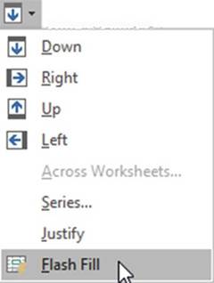
Figure 10-18. Select Flash Fill
Flash Fill used the three
columns of data along with the additional text you typed.
It even put the dollar
sign in front
of each of the amounts.
See Figure 10-19.
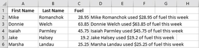
Figure 10-19. Result of Flash Fill
This exercise will show different features as
well as showing a potential problem that can arise when using Flash Fill.
1.
Open workbook Chapter 10 if it isn�t already opened.
2.
Click worksheet 3 Names.
3.
Figure 10-20 shows the data in the worksheet.
359
CHAPTER 10 ■ USING HYPERLINKS, COMBINING TEXT, AND WORKING WITH THE
STATUS BAR
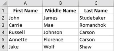
Figure10-20.Dataontheworksheetnamed3Names
We want to combine the individual�s first and last name.
4.
In cell D2 type John
Studebaker and then press Enter. Widen
the column to fit the name.
5.
Click inside cell D3.
Instead of going through the process of clicking the Home page,
then clicking the Fill button
in the Editing group, and then selecting Flash Fill, we will use the shortcut
key for Flash
Fill: Ctrl + E.
6.
Press CTRL + e. Figure 10-21 shows the result.
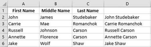
Figure10-21.ResultofusingFlashFill
You need to be careful about your spelling
which will be illustrated in the steps below.
7.
Select the data in column D. Right-click the selected data and select Clear Contents.
8.
In cell D2 type John Sludebaker and
then press Enter.
9.
Press CTRL + e.
Since Excel couldn�t find a match name in the
row it created the new name of Sludebaker for all of the copied cells. See Figure 10-22.
360
CHAPTER 10 ■ USING HYPERLINKS, COMBINING TEXT, AND WORKING WITH THE
STATUS BAR
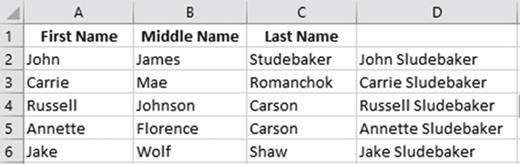
Figure 10-22.All of the last names in column D were
changed to Sludebaker
If you make a change to the end of the text, that change is reflected in the rows
below.
10.
Clear the contents in column D.
11.
In cell D2 type John Studebaker�s and
then press Enter
12.
Press CTRL + e. Figure 10-23 shows the results.
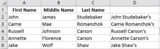
Figure10-23.ResultofchangingcellD2toJohnStudebaker�s
■
NoteIf we hadn�t
bolded or centered
the column headers
in columns A, B, and C, Excel
wouldn�t have known they were column headers.
This would have created a problem when we applied
Flash Fill. Excel
would have combined
the text in cell A1 and cell C1 and placed it into cell D1. This problem could
also be avoided
by putting a column header
in cell D1.
You don�t need to enter
the data from the columns
in the same order. We can easily
use the last name, followed
by a column, then a space, and then the first name.
13.
Clear the contents in column D.
14.
In cell D2 type Studebaker, John and then press Enter.
15.
Press CTRL + e. Figure 10-24 shows the results.
361
CHAPTER 10 ■ USING HYPERLINKS, COMBINING TEXT, AND WORKING WITH THE
STATUS BAR
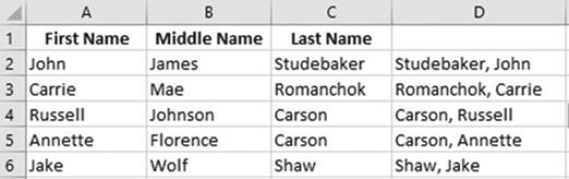
Figure10-24.ResultofchangingcellD2toStudebaker,John
The number of characters you type will be the number of characters that will be displayed from that column.
If you type the first
two letters in the name Studebaker then use Flash
Fill, Excel will display the first two letters of the other
last names.
See Figure
10-25
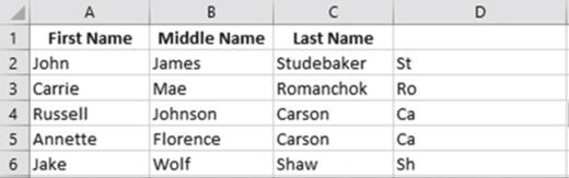
Figure 10-25.Typed
two letters in cell D2 so all the other
cells in column
2 display with two letters
The last name Shaw only contains four characters so if you enter more than four characters of the last name
the name Shaw will not appear at all. See Figure 10-26.
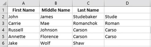
Figure 10-26.Shaw doesn�t
appear in column
D because it is only four characters
362
CHAPTER 10 ■ USING HYPERLINKS, COMBINING TEXT, AND WORKING WITH THE
STATUS BAR
Let�s show an example where we combine the individual�s first initial and
last name.
16.
Clear the contents in column D.
17.
In cell D2 type J. Studebaker and then press Enter.
18.
Press Ctrl + e. The results are
shown in Figure 10-27.
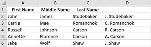
Figure10-27.ResultofenteringJ.StudebakerincellD2
Potential
Problem
In the second
row John and James both start with a �J,� which can cause some confusion. When there is a duplicate of text,
Excel
uses the left-most column. If we type John J. Studebaker and then use Flash Fill, Excel will use the initial
from column A rather than column B. See Figure
10-28.
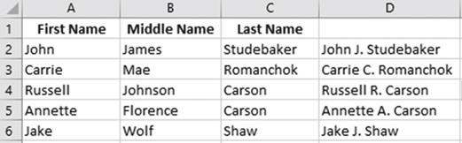
Figure 10-28.Result
of entering John J. Studebaker in cell D2
If we want to use the middle
initials we have to teach
it the correct pattern. We can
do this by typing the data from the next row(s) until
the pattern meets
our requirement. Since the middle name in row 3 doesn�t have the same initial as the first
name it will meet our needs.
1.
Clear the contents in column D.
2.
In cell D3 type Carrie M. Romanchok and then press Enter.
363
CHAPTER 10 ■ USING HYPERLINKS, COMBINING TEXT, AND WORKING WITH THE
STATUS BAR
3.
Press Ctrl + e. Figure 10-29 shows the results.
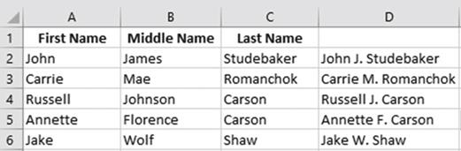
Figure10-29.ResultofenteringCarrieM.RomanchokincellD3
Using the Status Bar
The status bar at the bottom of your Excel
window can be used to display lots of useful
information. You can view computational results on different ranges without ever having to enter any
formulas. What is displayed on the status
bar is up to you. Right-clicking the status bar brings up all the available options,
as shown in Figure 10-30. You merely select
the options you want to see and deselect those
you don�t want to see. The selected
items appear with check marks
to the left of them.
Clicking anywhere on a line that has a check mark on it will remove the check mark.
Clicking anywhere on a line that doesn�t
have a check mark will place a check mark on it.
In this section, we�ll look at most of the options. We�ll
omit Signatures, Information Management Policy, and Permissions because these options are used only when
dealing
with SharePoint.
364
CHAPTER 10 ■ USING HYPERLINKS, COMBINING TEXT, AND WORKING WITH THE
STATUS BAR
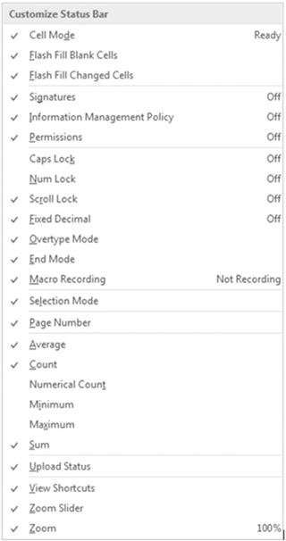
Figure10-30.AvailableoptionsontheStatusBar
365
CHAPTER 10 ■ USING HYPERLINKS, COMBINING TEXT, AND WORKING WITH THE
STATUS BAR
Cell Mode
The Cell Mode is displayed
in the left-most position of the status
bar. It displays
one of three words: Ready, Enter, or Edit. Ready indicates
that the cell is ready for you to enter data into. If you are entering
data into a cell, the word Enter appears.
If you double-click a cell to put it in edit mode, then the word Edit will appear.
Flash Fill Blank Cells
and Flash Fill Changed Cells
If these options
are turned on whenever you do a Flash Fill, the status bar will display the number of Blank
cells and the number of cells Flash Fill changed.
Using the data in Figure 10-31, if you typed Rhianna Slager in cell D1 to show Excel the
pattern, selected the cell range D1:D4, and then pressed
CTRL + e to start Flash Fill, there would be
one blank cell and two cells would have changed
which would show on the status
bar as

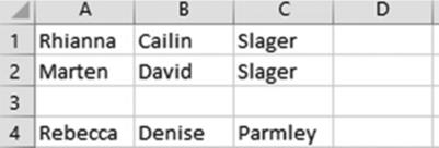
Figure 10-31. Original data entered
The resulting spreadsheet would look like
Figure 10-32.
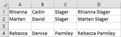
Figure10-32.ResultofusingFlashFill
Caps Lock, Num Lock
The words Caps Lock or Num Lock will display if they are turned on.
Scroll Lock
The words Scroll Lock will display
if Scroll Lock is turned
on. Scroll Lock is helpful
when you want to scroll through your worksheet but you want to keep track of your current
location. When Scroll
Lock is on, using your arrow keys moves your worksheet in the direction of the arrow,
but the active
cell doesn�t change.
366
Fixed Decimal
CHAPTER 10 ■ USING HYPERLINKS, COMBINING TEXT, AND WORKING WITH THE
STATUS BAR
This indicates when Fixed Decimal mode is
on.
Overtype Mode
Pressing the Insert key turns on Overtype
Mode. If Overtype
Mode is turned on and you are editing data in a cell, characters that you type will replace
existing characters; otherwise, existing characters will move over as you insert new characters.
End Mode
This displays when the End key has been pressed.
The End key is often used as part of a two-key combination.
Macro Recording
The Macro Recording
displays the button
 �on the status
bar when a macro is being recorded. Clicking the button stops the recording.
�on the status
bar when a macro is being recorded. Clicking the button stops the recording.
Selection Mode
The Selection Mode is used for selecting
cells with your arrow keys rather than dragging across them with your mouse.
Page Number
The Page Number
displays the current
page number and total number
of pages. The Page Number
only displays in Page Layout view.
Average,
Count, Numerical Count, Minimum, Maximum, Sum
These options instantly
display the result of calculations performed on the cells you select. The selected cells do not have to be
adjacent.
These math functions
are called Aggregate
functions. Aggregate functions
perform a calculation on a set of values and return a single value.
View Shortcuts
These three buttons
 �appear on the right side of the task bar. They control
how the worksheet is viewed. In order, they are the Normal view,
Page Layout view,
and Page Break
Preview.
�appear on the right side of the task bar. They control
how the worksheet is viewed. In order, they are the Normal view,
Page Layout view,
and Page Break
Preview.
367
CHAPTER 10 ■ USING HYPERLINKS, COMBINING TEXT, AND WORKING WITH THE
STATUS BAR
Zoom and Zoom Slider
The Zoomoption shows the current zoom percentage. The ZoomSlidercontrols the amount of
Zoom.

The Zoom tool is located
on the status bar at the bottom
right corner of your Excel
window. You can drag the Zoom tool�s
slider to the right to zoom in on objects
(make them larger)
or you can drag the slider to the left to zoom out on objects (make
them smaller). The zoom range
goes from 10% to 400%.
Not only is this
a great tool when you are developing your worksheets, but it also makes a great presentation tool.
In addition to dragging
the slider to change the zoom ratio,
you can also do the following:
�
Click anywhere in the slide range and the slider will move to that position.
�
Each time you click the Zoom out button
 �objects will decrease
by 10% in size.
�objects will decrease
by 10% in size.
�
Each time you click the Zoom in button
 �objects will increase
by 10% in size.
�objects will increase
by 10% in size.
■
Note� Changing the zoom ratio only affects your worksheet. It doesn�t change the
size of your ribbon.
This exercise covers the status bar options.
1.
Open the workbook Chapter 10 if it isn�t already open.
2.
Click the worksheet Status.
3.
Figure 10-33 shows the data in the worksheet.
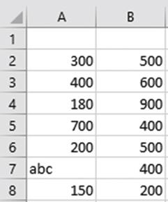
Figure10-33.DataintheworksheetnamedStatus
368
CHAPTER 10 ■ USING HYPERLINKS, COMBINING TEXT, AND WORKING WITH THE
STATUS BAR
Computations
1.
Right-click the
status bar. Select Average,
Count, Numerical Count, Minimum, Maximum, and Sum.
2.
Click an empty cell to close the status bar menu.
3.
Drag across cells A2 through
A8. Look at the result on your status bar. Your results
should look similar
to those in Figure 10-34.

Figure10-34.Computationsdisplayedonstatusbar
■
Note� Empty fields are excluded from computations and cell counts.
The difference between
Count and Numerical
Count is that Numerical Count only counts cells that contain numeric
data; therefore it excluded counting
the cell that contained the text abc.
4.
Right-click the status bar. Notice that the results are also displayed on the menu. See
Figure 10-35.
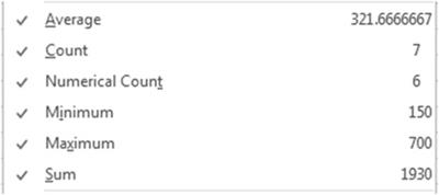
Figure 10-35.Results of selection are displayed on the Status
Bar menu
■
Note� The cells you select do not need to be vertical, in fact they don�t even need
to be adjacent to each other.
5.
Select cells A2:B8.
Look at the results.
6.
Click a blank cell to remove the selection.
7.
Hold down the
Ctrl key and select cells A2, A4, and
B6. The status bar now shows the
results for only these three cells.
Selection
Mode
1.
Click cell A2. Press F8. This makes
cell A2 the starting or anchor cell.
The status bar displays Extend Selection.
2.
Click cell B9. This highlights
all cells between the anchor cell and the selected cell.
369
CHAPTER 10 ■ USING HYPERLINKS, COMBINING TEXT, AND WORKING WITH THE
STATUS BAR
3.
Press the right arrow twice. This
extends the selection two columns.
4.
Press the down arrow key twice. This
extends the selection two rows.
5.
Click cell F15. This extends the
selection from the anchor point to cell F15.
6.
Use your arrow keys to move the selection back so that the
range A2:B9 is selected.
7.
The Shift + F8 key can be used to add additional ranges or individual cells to your current
selection. Press Shift + F8. The text on the status bar changes
from Extend Selection to
Add to Selection.
8.
Drag across cells E2:G9.
9.
Drag across cell B13:B16.
10.
Randomly click individual cells. They
will all become part of the selection.
11.
Press Shift + F8 to return to normal mode.
Cell Mode
1.
Click cell A17. If Cell Mode is selected you should see the word Ready on the far left side
of the status bar. If you don�t,
right-click the status bar and select Cell Mode.
2.
Start typing in the cell. The text should change from Ready to Enter.
After you finished
entering something in the cell press the Enter key.
3.
Double-click cell A17 to go into Edit mode. The text on the status
bar should now change to Edit.
You can now make any changes you want to the text in cell A17.
Caps
Lock, Num Lock, Scroll Lock
1.
Right-click the status bar and select Caps Lock, Num Lock, and Scroll Lock if they are not already
selected.
Click a cell to close the Status Bar menu.
The status bar will show when these keys are turned on. When they aren�t turned
on, nothing will appear. These
keys usually have lights associated with them on the keyboard
to give you a visual
clue as to whether they are on or not. Selecting these
gives you one more visual
clue.
2.
Click each of these keys to see how they appear on the
status bar and then click the keys again to turn them off.
Overtype
Mode
1.
Right-click the status bar and then select Overtype Mode if it isn�t
already selected.
2.
Misspell the word Excelin both cell A10 and cell A11 by leaving out the letter c (Exel). If
you see the word Overtypeon the status bar, click the Insert key to turn it off.
370
CHAPTER 10 ■ USING HYPERLINKS, COMBINING TEXT, AND WORKING WITH THE
STATUS BAR
3.
Double-click inside cell A10 to go into edit mode.
Place your cursor
between letters x and e. Now type the letter
c. The letter c should
insert and the letters e and l are moved to the right. Press
Enter.
4.
Double-click
inside cell A11 to go into
Edit mode. Place your cursor between the letters x and e. Press the Insert key. You should now see
Overtype on the status bar. Now type the letter c. It overtypes the letter e. The letter l doesn�t
move over. Overtyping prevents the insertion of characters. Press the Insert key. You should no
longer
see Overtype on the status bar.
5.
Type the letter e and press Enter.
Zoom, Zoom
Slider
1.
Drag the Zoom Slider bar to the right to increase the size
of items on your worksheet.
2.
Drag the Zoom Slider bar to the left to decrease the size
of items on your worksheet.
3.
Click the plus sign several times. Notice it increases the size by 10% every time you click it.
4.
Click the minus sign several times. It decreases the size by 10% every time you click it.
5.
Click the Ribbon�s
View tab. In the Zoom group, click
the Zoom button.
Select Custom. Enter 147 for the percent.
Click the OK button.
6.
In the Zoom group click the 100% button.
7.
Select cells A2:B8. Click the
View tab on the Ribbon.
8.
In the Zoom group, click the Zoom to Selection button. Using the Zoom to Selection makes
whatever is selected take up the size of the window either vertically or horizontally whichever
meets its limit first.
9.
Click in the center of the Zoom Slider to return to a 100% view.
Summary
Hyperlinks
can be used to create
quick links to files, web pages, a particular cell,
a new document, or an e-mail address.
You can combine data by using either Concatenation or Flash Fill. The & (ampersand) sign is used to
tie different strings of data together when using concatenation. Flash Fill can connect data automatically
without
having to manually
type the formula.
Users often forget about the status bar. This is probably because
the options aren�t visible unless you right-click it. The status bar is the fastest
way to view the results
of multiple functions
applied to multiple
ranges at the same time. The results
displayed on the status bar are temporary; they are not stored in cells.
In the next chapter you will learn
the different methods
of copying and pasting data.
You will also see how to switch
row and column
headings. You�ll learn
how to use the Microsoft Office Clipboard and how to key
data into multiple
worksheets at the same time.
371
CHAPTER
11
Transferring
and Duplicating Data to Other Locations
There are times when you
place data into cells and then later decide that you would rather display that data in a
different location, or maybe you want that data duplicated elsewhere. Excel
provides a variety of
methods for doing this as
well as allowing for you to select the format of the newly transferred or
duplicated data. This transferred or
duplicated data can be copied to locations within other data, in other
worksheets and in other workbooks.
After
reading and working
through this chapter
you should be able to
�
Move and copy cells using the drag-and-drop
method
�
Copy and paste manually
�
Copy and paste using the keyboard
�
Copy data to other worksheets
�
Copy data from one workbook to another
�
Use Paste Special
to transpose rows and columns
�
Use the Paste button gallery
�
Use the Add and Multiply option of Paste
Special
�
Use the Skip Blanks option of Paste Special
�
Use the Microsoft Office Clipboard
�
Insert copied or moved cells
Moving and Copying
Data
You can move data using Excel�s move feature also known as the cut feature. Moving a
cell moves the value in one cell to another cell. After the move the original cell location will be empty.
Any existing values in the receiving location will be overwritten by the moved data.
You may want to
have the same data in multiple locations. Rather than typing that same data
over and over again you can use
Excel�s copyfeature. Copyinga
cell involves copying the value in a cell to another cell. After the copy the value will
exist in both the original location and the location to where the value was copied. Whenever you cut or copy
data,
a duplicate of that data is placed in the Microsoft Office Clipboard. The clipboard is shared with other
Microsoft Office products. If you copy cells and then start Word and open
373
CHAPTER 11 ■ TRANSFERRING AND DUPLICATING DATA TO OTHER LOCATIONS
its clipboard, you will see the cells that you copied in Excel. You can then paste that cell data into your
Word document.
Moving a cell can be accomplished by using drag and drop or using the cut-and-paste method.
Copying can be accomplished by using drag and drop while holding
down the Ctrl key or using the copy- and-paste method.
Moving and Copying Cells
Using the Drag-and-Drop Method
When moving data using the drag-and-drop method
follow these steps:
1.
Select an area to be moved.
2.
Move the mouse cursor on one of the selected areas sides. The cursor should
turn into a move arrow, as shown in Figure Figure 11-1.
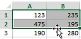
Figure 11-1. Select area to be moved.
3.
Drag the data to its new location. As you drag the data, a box the size of
the selected area moves with
the cursor so that you always know where the data will be moved.
See Figure 11-2.
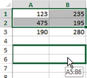
Figure 11-2.As you drag the data,
a box the size of selected area moves with the cursor.
4.
Release the mouse button. The data is moved to its new location. Any formatting that was applied
to a cell is moved with the value. See Figure 11-3.
374
CHAPTER 11 ■ TRANSFERRING AND DUPLICATING DATA TO OTHER LOCATIONS
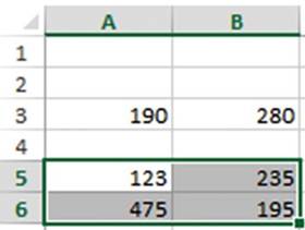
Figure 11-3. Result of moving data
When
copying data using the drag-and-drop method follow these steps:
1.
Select an area to be copied.
2.
Hold down the Ctrl key and move the mouse cursor on one of the selected
areas sides. The cursor should turn into an arrow with a plus sign. The plus
sign means you are copying the selected data. See Figure 11-4.
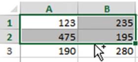
Figure 11-4. Select area to be moved.
3.
Keep the Ctrl key held down and drag the data to its new location. As you
drag the data, a box the size of the selected area moves with the cursor so
that you always know where the data will be copied. See Figure 11-5.
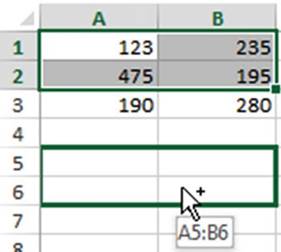
Figure 11-5.As you drag the data,
a box the size of selected area moves with the cursor.
375
CHAPTER 11 ■ TRANSFERRING AND DUPLICATING DATA TO OTHER LOCATIONS
4.
When the box is where you want it, release the mouse button. The data is copied
to its new location. Any formatting that was applied to a cell is copied along with the value. See Figure
11-6.
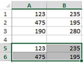
Figure 11-6. Result of copying data
■
Note� Cell references are automatically adjusted
when copying cells but not when moving them. You will
need to manually adjust cell references for moved cells and any cells that pointed to them.
Moving and
Copying Cells Using
the Cut and
Copy Buttons
The buttons for copying and pasting are located on the Home tab in the Clipboard group. See Figure 11-7.
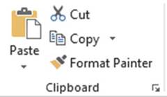
Figure 11-7. Ribbon�s Clipboard
group
To move
cell values
1.
Select the cells you want to move.
2.
Click the Cut button
 .
.
3.
Select the upper-left cell of where
you want the contents moved.
Click the Paste button.
376
CHAPTER 11 ■ TRANSFERRING AND DUPLICATING DATA TO OTHER LOCATIONS
To copy
cell values
1.
Select the cells you want to move.
2.
Click the Copy button
 .
.
3.
Select the upper-left cell of where
you want the contents copied.
Click the Paste button.
Rather than using Cut, Copy, and Paste buttons on the Ribbon, you can select them from the context
menu by right-clicking the selected cells.
■
Note� Excel displays an animated marquee
around cells that have been cut or copied. After you have finished pasting
the contents to their new location cancel the animated
marquee by pressing
the Esc key.
Moving and Copying
Cells Using the Keyboard
It�s impossible
to remember all the keyboard shortcuts, but you should remember the ones for
copying, cutting, and pasting since you will be using these all the time. See Table
11-1.
Table 11-1. Keyboard Shortcuts

Function��� Shortcut Keys
Cut����� Ctrl + X
Copy���� Ctrl + C
Paste���� Ctrl + V

These
same shortcuts are used in most other programs as well.
In this exercise, you duplicate cell content by using copy and paste and then
move content using cut and paste.
1.
Start a new workbook named Chapter 11. Name
the worksheet �CopyPaste.�
2.
Enter the data in Figure
11-8 into a worksheet.
377
CHAPTER 11 ■ TRANSFERRING AND DUPLICATING DATA TO OTHER LOCATIONS
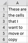
Figure 11-8. Enter this data.
Duplicate
Cell Contents

1.
Select cells A1:A6.
2.
On the Home tab in the Clipboard group, click the Copy button�� to copy the contents of cells
A1:A6.
Pressing Ctrl + C is the shortcut
key for the Copy command.
An animated marquee appears around cells
A1:A6 to indicate that these cells are being copied.
3.
Click inside cell C3. This is
the upper-left cell of where the content will be copied to.
4.
On the Home tab in the Clipboard
group, click the top half of
the Paste button
 . A duplicate copy of the contents in cells A1:A6 now exists in
cells C3:C8.
. A duplicate copy of the contents in cells A1:A6 now exists in
cells C3:C8.
5.
As long as the animated marquee
appears around the cells being copied you can continue to paste them in other
locations.
Click
inside cell C7. This
time use the paste shortcut Ctrl + V instead of using the Paste button. When you paste content
into cells that already have content, the original contents are copied over.
6.
Press the Esc key. The animated
marquee is removed.
Move
Cell Contents

1.
Select cells A1:A6.
2.
On the Home tab in the Clipboard group, click the Cut button�� to cut the cells. Pressing
Ctrl + X is the shortcut key for the Cut command.
3.
Click inside cell E1. This is
the upper-left cell of where the content will be moved to.
4.
Press Ctrl + V to paste the contents to their new location. The cell contents
have been moved to cells E1:E6. The animated marquee
has been removed.
You have
learned how to move and copy cell data by using the drag-and drop method, using
keyboard shortcuts, and clicking the
Cut and Copy command buttons. These methods didn�t provide any options for specifying what to paste and how
to
format it. If you want a choice as to how the pasted data is to appear, you will
need to make your selection from the Paste Button Gallery. The Paste button
gallery is accessed by clicking the bottom half of the Paste button.
378
Paste Button Gallery
CHAPTER 11 ■ TRANSFERRING AND DUPLICATING DATA TO OTHER LOCATIONS
The Paste button is actually two separate buttons.
If you let your cursor set on the top half of the Paste button you will see the tooltip shown on the left
side of Figure 11-9. If you let your cursor set on the bottom half of the Paste button (the half with the
down arrow) you will see the tooltip on the right side of Figure 11-9. Clicking the bottom portion
of the Paste button highlights the entire button and presents
a gallery of paste options.
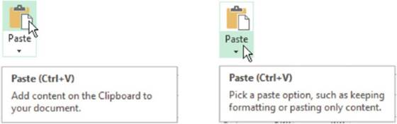
Figure 11-9.Paste by clicking
the top of the button,
or open the Paste gallery
by clicking the lower half of the button.
The paste
options in the gallery can perform such functions as pasting only the
formatting rather than the
data or pasting the results of formulas and not the formulas themselves. Figure
11-10 shows the Paste gallery options. Not all of the
options appear every time; it depends upon what you copied. Table 11-2 displays each paste option and a
description for it.
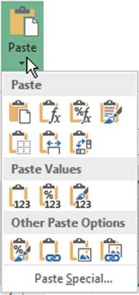
Figure 11-10. Paste options
379
CHAPTER 11 ■ TRANSFERRING AND DUPLICATING DATA TO OTHER LOCATIONS
Table11-2.ThePasteGalleryOptions

Button���� Name
with Shortcut Key������ Description

Paste (P)���������� Paste
everything exactly as is from the original
copy. Keeps all the formatting, formulas, etc. Doesn�t
adjust column widths.

Formulas (F)�������� Pastes everything except the
formatting

Formula & Number Formatting (O)� Pastes formulas & number
formatting such as
dollars signs, commas, negatives in parentheses,
etc., but does not copy text formatting.

Keep Source Formatting (K)��� Pastes all
the data along with all the formatting.

No Borders (B)������� Pastes everything except any
borders that were applied to the copied
cells

Keep
Source Column Widths (W)�� Pastes everything and adjusts the column widths to
match those that were copied.

Paste Values


Transpose��������� Changes the orientation of the copied cells. For example, if the copied cells were in a
vertical format they would be change to a horizontal format.
Values (V)��������� Only the values are
pasted not the
formulas. No formatting is pasted.
Values & Number Formatting (A)�� Pastes only the results
of formulas not the formulas
themselves. Pastes
any numeric formatting such as
$ and commas,
etc., but not any text formatting.
Values & Source Formatting (E)�� Pastes only the results
of formulas, not the
formulas themselves. Pastes all the formatting applied
to the original copied cells.
Other
Paste Options

Formatting (R)������� Pastes only the formatting applied to the
cells, not the data itself.

Paste Link (N)������� Creates a link to the copied item. Pasting a link means the pasted cell will always be
updated when you change the original cell.

Picture (U)�������� Pastes your data as a picture rather than individual cells of data. The pasted data can�t
be edited.

Linked Picture (I)������� Pastes everything. Any changes you make to the original data or its formatting is
automatically updated in the pasted data.
380
CHAPTER 11 ■ TRANSFERRING AND DUPLICATING DATA TO OTHER LOCATIONS
In this exercise you will apply the various paste options to see how they
affect your data.
1.
Use the Chapter 11 workbook you created. Create a new worksheet named �Pasting.�
2.
Type Jan in cell A1. Press Ctrl + Enter.
3.
Drag the AutoFill Handle to the
right until you have the months Jan through May.
4.
Select Cells A1:E1. On the
Home tab
in the
Font group
click the
Increase
Font Size
button three times. Change
the font
color to
Red.
Change the fill color to
(Green, Accent 6, Lighter
80%).
Bold and center the headings.
5.
Enter the rest of the data in Figure 11-11.
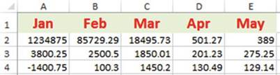
Figure11-11.Entertherestofthisdata.
6.
Apply AutoSum to cells A5:E5.
7.
Select cells A2:E4.
On the Home tab, in the Number group, click
the Comma Style button.
8.
Select cells A5:E5. On the Home tab, in the Number group, click
the
 �button.
9.
On the Home tab, in the Font group, click the down arrow for borders. Select
Top and Double Bottom border.
10.
Select column heads
A through E. Double-click between
column heads E and F to AutoFit
the column width
as shown in Figure 11-12.
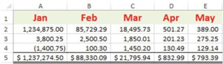
Figure 11-12. AutoFit the column width.
11.
Select cells K1 and K2. Apply bold, italic, and underline
to the cells.
381
CHAPTER 11 ■ TRANSFERRING AND DUPLICATING DATA TO OTHER LOCATIONS
View how
Paste Options Affect the Copied Data
1.
Select cell A1:E5.
Press Ctrl + C.
2.
Click inside
cell G1. Click the bottom half of
the Paste button so that you can see the
gallery of paste options.
3.
Move your cursor over the paste options. The results should appear as those in the table.

Paste Option�����������������
Example
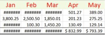
 �Paste
Pastes all the data and formatting but doesn�t adjust the columns widths to match those being copied. This is
the same as pressing
Ctrl + V.
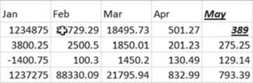
 �Formulas
Pastes the data and the formulas. Doesn�t paste
any formatting. The formatting that exists in the
pasted area will affect the copied cells (Notice the formatting in cells K1 and K2)
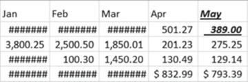
 �Formula & Number Formatting
Pastes formulas and only number formatting,
no other formatting. The formatting that exists
in the pasted area will affect the copied cells.
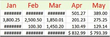
 �Keep Source Formatting
Preserves the look of the original
data except it doesn�t adjust column widths.
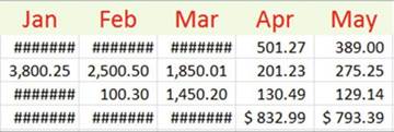
 �No Borders
Notice the top and double
bottom borders weren�t pasted
(continued)
382
CHAPTER 11 ■ TRANSFERRING AND DUPLICATING DATA TO OTHER LOCATIONS
Paste
Option����������������� Example
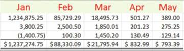
 �Keep Source Column Widths
Looks like the original
including maintaining the column
widths
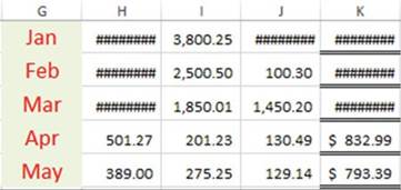
 �Transpose
Changes the orientation of the rows and
columns
 �Values

 �Values & Number
Formatting Values &
Source Formatting
�Values & Number
Formatting Values &
Source Formatting
None of the formatting is copied over.
It displays the results of the formulas
but doesn�t keep the formulas.
Looks the same As Formula & Number Formatting. It
doesn�t preserve formulas; rather it displays the results of the formulas.
Looks the same as Keep Source Formatting. It doesn�t preserve formulas; rather it displays the results of the
formulas.
4.
With the copy area A1:E5
still selected, click
inside cell G1. Click the down arrow portion of the Paste button. In the Other Paste Options area
click the Formatting button
 . All the formatting has been pasted
but none of the cell contents. See Figure 11-13.
. All the formatting has been pasted
but none of the cell contents. See Figure 11-13.
Figure11-13.Formattingpastedwithoutcellcontents
5.
If you type data in one of the cells in the pasted area, the data will take on the formatting of
the original copied cell:
a.
Type June in cell G1.
b.
Type 395 in cell G5.
383
CHAPTER 11 ■ TRANSFERRING AND DUPLICATING DATA TO OTHER LOCATIONS
6.
Select cells G1:K5. On the Home tab, in the Editing group,
click the Clear button and select Clear
All. Selecting Clear
All clears the data and all formatting.
7.
Select cells A1:E5.
Press Ctrl + C. Click
inside cell G1. Click the bottom half of the Paste button.
In the Paste Values
area click the Values button
 . Click inside cell G5. Notice in the formula
bar that there is no formula but only the result of the formula
used in the copied cell.
. Click inside cell G5. Notice in the formula
bar that there is no formula but only the result of the formula
used in the copied cell.
8.
Select cells G1:K5. On the Home tab, in the Editing group,
click the Clear
button and select
Clear All.
9.
Select cells A1:E5. Press Ctrl
+ C. Click
inside cell G1. Click
the bottom
half of
the Paste
button. In the Other Paste
Options area click the Paste
Link button. The pasted area is linked
to the
copied area. Any changes you
make in
the copied
area will
be reflected
in the
pasted area.
10.
Click inside cell G2. Cell
G2 contains the formula =A2. Cell G3 contains the formula =A3.
11.
Change the value in cell A3 from 3,800.25 to 6,725.50. The change is reflected in cell G3. The
total in cell G5 was changed so that it has the same value as cell A5.
12.
Select cells G1:K5. On the Home tab, in the Editing group,
click the Clear
button and select
Clear All.
13.
Select cells A1:E5. Press Ctrl + C. Click inside cell G1. Click the bottom half of the paste
button. In the Other Paste Options area click the Picture button. The pasted
area is treated as an image. You can tell that it is now an image because the
contextual tab group Picture Tools displays with its Format tab.
14.
Click the Format
tab. You can move your cursor across the Picture
Styles to see how they would affect the image.
Click the down arrow for the Picture
Styles to see more choices.
15.
Press the Delete key remove the image
in cell G1.
16.
With cells A1:E5
still selected, click inside cell G1. Click
the bottom half of the paste button.
In the Other Paste Options area
click the Linked Picture button.
Notice
the contextual tab group Picture Tools is visible
again. Since the image is linked to the copied cells any changes you make to the original,
cells will be reflected in the pasted image.
17.
Change the value in cell D3 to 87.75. The change is reflected in the pasted
image.
18.
Change the font color in cell A1 to blue. Italicize
cell A1. Notice the change in the pasted
area.
19.
Close the Chapter
11 workbook.
You have used Paste options to copy cell values, cell formats, formulas only, and other formatting. Next,
you will learn how to copy data from one worksheet to another and then later how to copy data from one
workbook to another.
384
CHAPTER 11 ■ TRANSFERRING AND DUPLICATING DATA TO OTHER LOCATIONS
Copy Data to Other Worksheets Using Fill Across Worksheets
You can copy all or a portion of the data on one worksheet to other worksheets by using the Fill Across
Worksheets copy command. The following steps are used to perform the Fill Across Worksheets copy
command:
1.
Select the cells that you want copied to the other worksheets. You can only select the entire
worksheet or a single range. If you want to copy multiple ranges, then you will need to repeat the steps.
2.
Select the worksheet tabs of the worksheets where
you want the data copied.
3.
On the Ribbon, on the Home tab, in the Editing group, click the Fill
button. Choose Across Worksheets. The Fill Across Worksheets dialog box opens.
Here you can select if you want to copy
everything, only the data, or only the
formatting.
In this exercise you will copy data from one worksheet to other
worksheets.
1.
Create a new workbook named Chapter 11B.
2.
Create two new worksheets so that you have tabs for Sheet1, Sheet2,
and Sheet3
3.
Enter the Data in Figure 11-14 in Sheet1 and format as follows:
a.
Widen column B so that all the text fits in the column.
b.
Bold and italicize the title Chart of Accounts. Change
the size of the title font to 16. Merge
and center the title.
c.
Apply a fill color of Green, Accent
6, Lighter 40% for the title.
d.
Click cell B3. Hold
down the Ctrl key while
you click cell A12
and A17. Click Bold and then Center
for the Alignment.
385
CHAPTER 11 ■ TRANSFERRING AND DUPLICATING DATA TO OTHER LOCATIONS
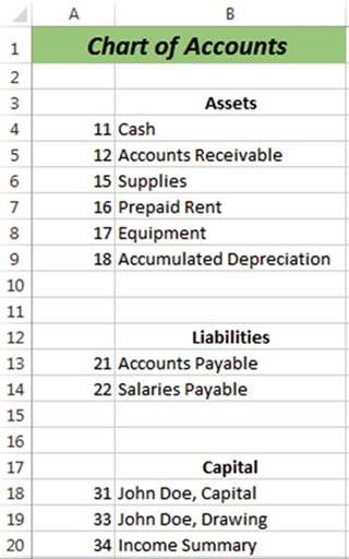
Figure 11-14. Enter this data.
4.
Select cells A3:B9
5.
Hold down the Ctrl key and click the Sheet2 tab and Sheet3
tab at the bottom of the worksheets.
6.
On the Ribbon,
on the Home tab, in the Editing
group, click the Fill button.
Choose Across Worksheets. See Figure 11-15.
386
CHAPTER 11 ■ TRANSFERRING AND DUPLICATING DATA TO OTHER LOCATIONS
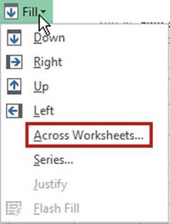
Figure11-15.SelectAcrossWorksheets
The Fill Across Worksheets dialog box opens. See Figure 11-16.
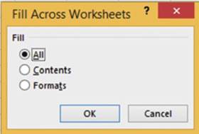
Figure11-16.FillAcrossWorksheetsdialogbox
You can select if you want to copy everything, only the data, or only the formatting.
7.
Select All and click the OK button.
8.
Right-click one of the worksheet tabs.
Select Ungroup Sheets.
9.
Click the Sheet2 tab. You
will notice that the column widths didn�t automatically adjust to the copied
data.
10.
Adjust the column widths on Sheet2 and Sheet3.
Copy Data from One Workbook
to Another
You can copy data from one workbook to another by copying the data from one workbook
and then pasting
it into another
workbook using one of the paste methods.
387
CHAPTER 11 ■ TRANSFERRING AND DUPLICATING DATA TO OTHER LOCATIONS
This exercise covers using the various paste options when copying data.
1.
Use the workbook Chapter 11B that you created in the previous exercise.
2.
Press Ctrl + N. This is the
shortcut key to create a new workbook.
3.
On the Ribbon,
on the View tab, in the window
group click the Arrange All button. The Arrange Windows
dialog box displays.
See Figure 11-17.
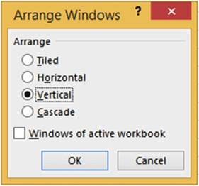
Figure11-17.ArrangeWindowsdialogbox
4.
Select Vertical. Click the OK button.
5.
Select all of the data on Sheet1 of the Chapter 11B workbook. Press Ctrl + C to copy the data.
6.
Click inside cell A1
of the new workbook. Press Ctrl + V to paste the data into the new workbook.
The column widths of the pasted data does not match the
column widths of the copied data.
7.
Click the Paste Options button
 �that appears at the bottom right of the pasted date or click the Ctrl key to bring up the Paste
Options.
See Figure 11-18.
�that appears at the bottom right of the pasted date or click the Ctrl key to bring up the Paste
Options.
See Figure 11-18.
388
CHAPTER 11 ■ TRANSFERRING AND DUPLICATING DATA TO OTHER LOCATIONS
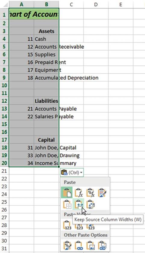
Figure 11-18. Paste options
389
CHAPTER 11 ■ TRANSFERRING AND DUPLICATING DATA TO OTHER LOCATIONS
8.
Click the Keep Source Column Widths button. The
columns adjust to their original width.
Let�s repeat what we have just done, but this time we will copy the entire
worksheet.
9.
Let�s start by clearing the data we pasted into the new workbook. Press Ctrl + Z.
10.
Select all of the data on Sheet1 of the Chapter 11B workbook by clicking the Select All button to
the left of the column A header. Press Ctrl + C.
11.
Click
cell A1 of the new workbook.
12.
In the Clipboard group click the bottom half of the Paste
button. The Paste button gallery is displayed.
13.
Move your cursor over the different buttons; as you do so
you will see exactly how the spreadsheet would look if you clicked that button.
Since you had the entire worksheet selected,
the Paste button and the Keep Source Column Widths button give the same results.
14.
Click the Paste button.
15.
Close the two workbooks.
Paste Special
The Paste Special command
provides even more control over your pasting.
It should be used whenever
you want to do any of the following:
�
Paste some of the properties from a copy or a cut cell operation.
�
Perform a mathematical operation using the contents from the copied
or cut cells with the pasted cell contents.
�
Ignore cell blanks.
�
Transpose
row data into column data or column
data into row data.
�
Link the pasted cells to the copied cells.
The
Paste Special command
is located at the bottom
of the Paste gallery. See Figure 11-19.
390
CHAPTER 11 ■ TRANSFERRING AND DUPLICATING DATA TO OTHER LOCATIONS
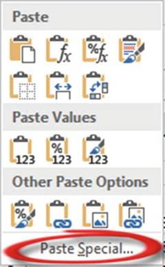
Figure11-19.SelectPasteSpecial.
Using Paste Special
Selecting Paste Special brings up the Paste Special dialog box. See Figure 11-20.
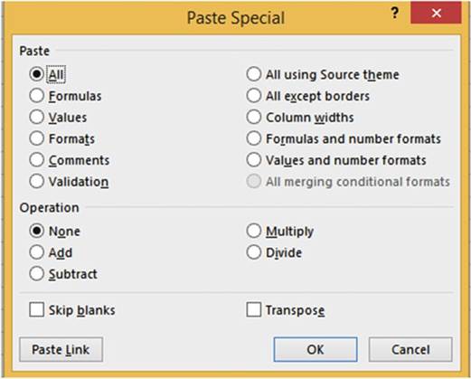
Figure 11-20. Paste Special dialog box
391
CHAPTER 11 ■ TRANSFERRING AND DUPLICATING DATA TO OTHER LOCATIONS
■
Note� The Paste Link button at the bottom
of the window is only available when All or All Except
Borders is selected. It is grayed
out when anything
else is selected.
Table
11-3 describes the Paste options. Table
11-4 describes the Operation options.
Table11-3.PasteSpecialOptions

Paste Special Option������ Description
All����������� This
performs the same operation as pressing Ctrl + V. It pastes all cell contents and formatting. It does not
adjust the column widths.
Formulas��������� Pastes the formulas used in the copied cells.
Values��������� Pastes only the results
of formulas, not the formulas
themselves.
Formats��������� Pastes only the formatting not the data.
Comments������� Pastes only comments attached to the cell.
Validation�������� Pastes data validation rules
for the copied
cells.
All Using Source Theme���� Pastes all cell contents and formatting using
the theme that was applied
to the copied cells.
All Except Borders�����
Pastes everything except any borders that were applied to the copied
cells.
Column Widths������
Pastes the columns widths so they match the width of the columns of
the copied cells.
Formulas and Number
Formats� Paste formulas and cell contents. Pastes any numeric
formatting such
as $ and commas, etc., but not any text formatting.
Values and Number
Formats�� Pastes only the results
of formulas, not the formulas
themselves. Pastes
any numeric formatting such as $ and commas, etc., but not any text
formatting.
■
Note� Depending upon the content you are copying
and the paste
options that you have selected, some options may be unavailable.
Table 11-4. Operation Options
Operation Option�� Description
None����� Do not perform any
mathematical operation to the pasted
cells.
Add����� Add the values in the copied cells to those in the pasted cells. Subtract�����
Subtract the values in the copied cells from those in the pasted cells. Multiply����� Multiply the values in
the copied cells to those in the pasted cells.
Divide����� Divide the values in the copied
cells into those
in the pasted
cells.
392
CHAPTER 11 ■ TRANSFERRING AND DUPLICATING DATA TO OTHER LOCATIONS
■
Note� Mathematical operations can only be applied to values. If you are performing
one of the mathematical operations (Add, Subtract, Multiply,
or Divide) you must select
either All, All except borders,
or Values and number formats
from the Paste options.
To use Paste Special:
1.
Select the cells that contain the data or attributes that you want to copy.
2.
Press Ctrl + C.
3.
Select the upper-left cell of the paste area.
If you are performing a mathematical operation
you will need to select
all the cells
in the paste area.
4.
On the Home tab, in the Clipboard, click the bottom
half of the Paste button.
Select Paste Special.
5.
Select the Paste option
you wish to perform.
6.
Select the Operation option you want to perform.
If you aren�t performing a mathematical operation select None.
7.
If you want to paste static data (not linked) click the Paste option you want to use and then
click the OK button.
OR
�
If you want to paste linked data, you must select either All or All except
borders
from
the Paste options
and then click
the Paste Link button.
�
Avoid copying blank cells to your paste area by selecting Skip blanks.
�
Change row data to columns
or vice versa
by selecting Transpose.
■
Helpful Hint� If you find yourself
using Paste Special
frequently you can add it to your Quick Access
Toolbar.
Using Paste Special
to Transpose Rows
and Columns
The Paste Special command
has a Transpose option that is used for converting row data to column data and vice versa. A likely scenario
in
which you would use the Transpose function is that you have set up your row and column headings and then
decide that what you really wanted was to have the row headings as the column headings and the column
headings as the row headings. Rather than manually retyping the headings, you can flip-flop them by
using Paste Special�s Transpose option.
In this exercise you will transpose the rows and columns of the original
copied data.
1.
Create a new workbook named Chapter 11C.
Name the worksheet �Transpose.�
2.
Enter the data in Figure 11-21. Bold the column headings.
393
CHAPTER 11 ■ TRANSFERRING AND DUPLICATING DATA TO OTHER LOCATIONS
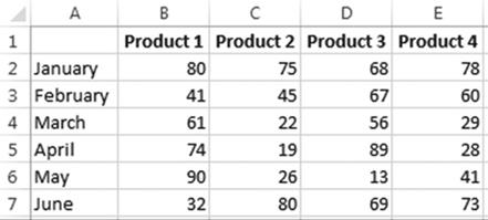
Figure 11-21. Enter this data.
3.
Select cells A1:E7
4.
Right-click the selected data and select Copy.
5.
Right-click inside cell A10. Select Paste Special from the context
menu.
6.
In the Paste area select Values (Figure 11-22). Selecting All would
leave what will now
become are row headings bolded.
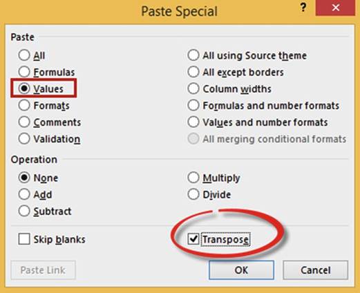
Figure 11-22.Select
values and Transpose
from the Paste Special dialog box.
7.
Select Transpose.
8.
Click the OK button.
9.
Bold and center the column
headings.
394
CHAPTER 11 ■ TRANSFERRING AND DUPLICATING DATA TO OTHER LOCATIONS
The result should be as shown in Figure 11-23.
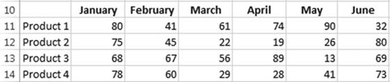
Figure11-23.Resultoftransposingrowandcolumnheads
Using Paste Special
to Perform Calculations
Paste Special can perform calculations while pasting. Paste Special has operation options for Add, Subtract,
Multiply, and Divide.
A single
cell value can be pasted
to a group of cells
while performing an arithmetic operation, or a group
of cells can be pasted
to another group
of cells while
performing an arithmetic operation.
Let�s say you want to add the value 5 in cell A3 to each of the cells in the range A1:D1. See Figure 11-24.
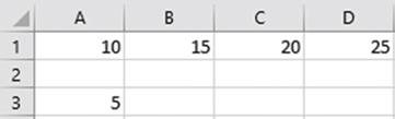
Figure11-24.YouwilladdthevalueincellA3toeachcellintherangeA1:D1.
You would perform the following steps:
1.
Select cell A3 and then do a copy.
2.
Select the cells
where you want to paste
the operation. In this case that would
be range A1:D1.
3.
Right-click one of the selected cells
and then select
Paste Special.
4.
Select the Add operation.
The result would be as shown in Figure 11-25 where 5 has been added to each value in the pasted range.
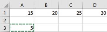
Figure11-25.Fivewasaddedtoeachcellinrow1.
395
CHAPTER 11 ■ TRANSFERRING AND DUPLICATING DATA TO OTHER LOCATIONS
You
can combine a group or multiple groups while performing an arithmetic operation.
If you wanted to add the individual values in row 3 to the individual values in row 1, as shown in Figure
11-26, you would perform the following steps:
1.
Select the cell range
A3:D3 and then do a copy.
2.
Select cells A1:D1
3.
Right-click one of the selected cells
and then select
Paste Special.
4.
Select the Add operation.
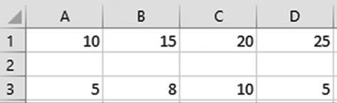
Figure11-26.Valuesinrow3willbeaddedtothoseinrow1.
Figure 11-27 shows the result.
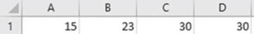
Figure11-27.Resultofaddingthevaluesinrow3torow1
If you were copying
fewer values than you were pasting, then the copied
values would repeat
their pattern.
In Figure
11-28 the value in cell A3 would be added to the value in cell A1. The value in cell B3 would be added to
the value in B1.
Then the value in cell A3 would be added to the value in C1, and the value in B3 would be added to the value
in D1.
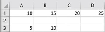
Figure 11-28.Value in cell A3 will be added
to cells A1 and C1. Value in cell B3 will be added to cell B1 and
D1.
Figure 11-29 shows the result.
396
CHAPTER 11 ■ TRANSFERRING AND DUPLICATING DATA TO OTHER LOCATIONS
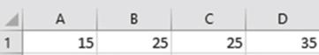
Figure 11-29.Value
in A3 was added to A1 and C1. Value in B3 was added to B1 and D1.
The Paste Special
option Add can be beneficial when you want to combine
groups of values.
The Add option adds the values
you copied in the source range
with those in the destination range and then replaces
the destination range
with the new values.
In this example,
we will combine the values
in Groups B and C with Group
A. We will then delete
the rows that contain the Group B and Group
C values.
1.
Open workbook Chapter 11C. Create
a new worksheet named �PasteAdd.�
2.
Create the spreadsheet as shown in Figure 11-30.
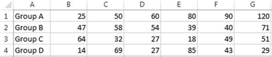
Figure 11-30. Enter this data.
3.
Select the cell range B2:G2 and do the following:
a.
Press Ctrl + C.
b.
Click inside cell B1. Click the lower half of the Paste button.
c.
Select Paste Special.
d.
Under Operation select Add. Click OK.
4.
Select the cell
range B3:G3.
Press Ctrl + C. Click
inside cell B1. Click the lower
half of
the Paste
button. Select Paste Special. Under Operation select
Add. Click OK.
5.
Select row heads 2 and 3 and then right-click and select
Delete from the context menu. See
Figure 11-31.
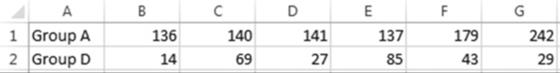
Figure11-31.Resultofdeletingrows2and3
The values in Group A are now the sum of the values that were previously in Group A plus Group
B plus Group C.
397
CHAPTER 11 ■ TRANSFERRING AND DUPLICATING DATA TO OTHER LOCATIONS
We have a list of prices for the items we sell. We want to increase the price for each product by 10%.
1.
Open the workbook Chapter 11C. Create
a new worksheet named �PasteMultiply.�
2.
Enter the data as shown in Figure
11-32.
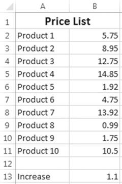
Figure11-32.EnterthisdatainworksheetPasteMultiply.
3.
Click cell B13. Press Ctrl + C.
4.
Select cell range B2:B11.
Right-click the selected cells and then select Paste Special from the context menu.
5.
Select Multiply under Operation. Click the OK button.
Excel Multiplies each value in the pasted
area by 1.1. Figure 11-33 shows the result.
398
CHAPTER 11 ■ TRANSFERRING AND DUPLICATING DATA TO OTHER LOCATIONS
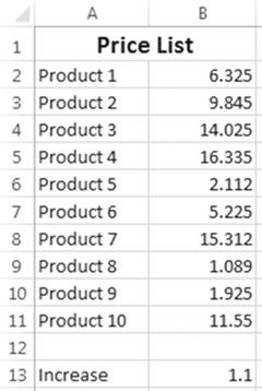
Figure 11-33.Result
of multiplying each value in the pasted area by 1.1
Experiment with the other Operation
options.
When you copy a range
of cells, any cells that are blank
in the copied range will overwrite any cells in the pasted
range, thus making those
cells also blank.
However, if you use the Skip Blanks option for Paste Special,
the blank cells in the copied range will not overwrite the data in the cells in the pasted range.
1.
Use the workbook Chapter 11C. Create
a new worksheet named �Skip.�
2.
Type the data as shown in Figure
11-34.
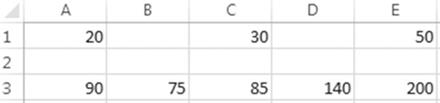
Figure 11-34. Enter this data.
3.
Drag across cells A1:E1. Press Ctrl + C to copy them.
4.
Click in cell A3. Press Ctrl + V. See Figure 11-35.
399
CHAPTER 11 ■ TRANSFERRING AND DUPLICATING DATA TO OTHER LOCATIONS
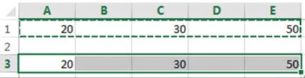
Figure11-35.CellRangeA1:E1pastedtorangeA3:E3
5.
Notice that the copied blank cells replaced those in cells B3 and D3.
6.
Press the Undo button on the Quick
Access Toolbar or press Ctrl + Z to undo the paste.
6.
Click the lower half of the Paste button.
Select Paste Special.
7.
Select Skip Blanks. Click OK. See Figure 11-36.
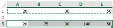
Figure 11-36.Used
Paste Special to prevent blank
cells from copying
over non-blank cells
The values in cells B3 and D3 have not
been changed.
Inserting Copied or Moved Cells
Rather than having a move or copy override the values in the receiving location you can insert the copied or
moved cells so that the values in the receiving location are moved to accommodate them.
Insert Copied Cells
The three steps to copying the cells in the range A1:B2 of Figure 11-37 to the cell range A6:B7 are as
follows:
400
CHAPTER 11 ■ TRANSFERRING AND DUPLICATING DATA TO OTHER LOCATIONS
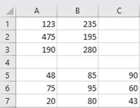
Figure 11-37.Copy
cells in range
A1:B2 to the cells in range A6:B7
Step 1
First select the cells that you want to copy. Right-click the selection and then select Copy from the context
menu. See Figure 11-38.
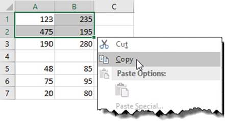
Figure 11-38.Right-click the selected cells and then select Copy.
Step 2
Right-click cell B6 and then select Insert Copied Cells from the context menu. See Figure 11-39.
401
CHAPTER 11 ■ TRANSFERRING AND DUPLICATING DATA TO OTHER LOCATIONS
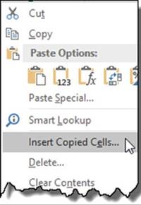
Figure11-39.SelectInsertCopiedCells.
Step 3
Select the direction in which you want the current cell values moved.
See Figure 11-40.
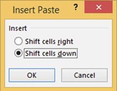
Figure 11-40.Select the direction in which want the
current cell values moved.
Figure 11-41 displays the result from Step 3 if you selected Shift cells down.
402
CHAPTER 11 ■ TRANSFERRING AND DUPLICATING DATA TO OTHER LOCATIONS
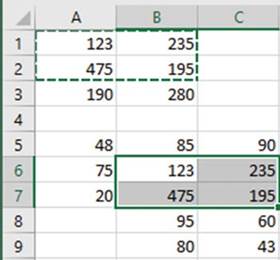
Figure11-41.ResultsifyouselectedShiftcellsdown.
Figure 11-42 displays the result from Step 3 if you selected Shift Cells right.
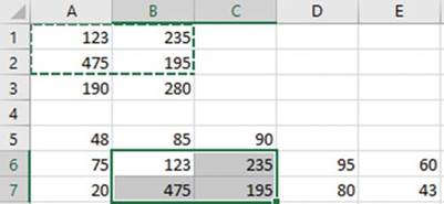
Figure11-42.ResultsifyouselectedShiftcellsright.
Insert Cut Cells
Inserting cut cells works similar to inserting copied cells.
In this exercise you will move data to
another location forcing the data that is currently in the receiving location
to move down into the cells below.
1.
Use the Chapter 11C workbook you created. Create a new worksheet named �CutCells.�
2.
Enter the data in Figure
11-43 into a worksheet.
403
CHAPTER 11 ■ TRANSFERRING AND DUPLICATING DATA TO OTHER LOCATIONS
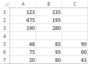
Figure 11-43. Enter this data.
3.
Select the cell range A1:B2. Press Ctrl + X to cut the cells for a
move.
4.
Right-click inside cell B5. Select
Insert Cut Cells. Figure 11-44 shows the result.
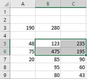
Figure11-44.Copieddataoverexistingdata
5.
Close the Chapter 11C workbook.
Using the Microsoft Office Clipboard
Whenever you do a Copy, the item you copied is placed into the Office
Clipboard. The Office
Clipboard is a temporary storage area to which you can copy as many as 24 items. The items can be text or
graphical such as charts, images, clip art, shapes, and so on. The clipboard is shared with the other
Microsoft Office products. This
means that you can copy and paste
items between Excel,
Access, PowerPoint, Word,
and so on. The clipboard makes it quick
and easy to rearrange data in your documents or to merge
elements from other
office
products into your documents. Items that are on the clipboard can be pasted
individually or all at once.
The items stay on the clipboard until you delete them from the clipboard or until you have closed all of the
Microsoft Office applications. The last item you added to the clipboard remains even after you have
closed all of the Microsoft Office applications. The last item copied is added to the top of the clipboard.
If you try to add more than 24 items to the clipboard, the first item you added will be removed. All items
are cleared when you restart your computer.
404
CHAPTER 11 ■ TRANSFERRING AND DUPLICATING DATA TO OTHER LOCATIONS
The clipboard can be opened
by clicking the Dialog Box Launcher for the clipboard group. This opens the Clipboard Task Pane.
This exercise covers copying text, shapes, images,
and charts using the clipboard.
1.
Open workbook Clipboard.xlsx.
2.
Click the Clipboard
worksheet tab.
3.
Click the Dialog Box Launcher for the Clipboard group to open the
clipboard pane.
4.
Click the Clear All button.
5.
Make the following selections:
a.
Select cells B3:C3. Press Ctrl + C.
b.
Select cells B4:C4. Press Ctrl + C.
c.
Select cells B5:C5. Press Ctrl + C.
d.
Select cells B6:C6. Press Ctrl + C.
6.
Click the Blank worksheet tab and complete the following steps:
a.
Click cell A2. Click Wolves
7 in the Clipboard pane.
b.
Click cell A3. Click Elephants
5.
c.
Click cell A7. Click the Paste All button.
d.
Click the Clear All button.
7.
Select the Clipboard Worksheet
tab and complete the following steps:
a.
Click the edge of the Shape. Press
Ctrl + C.
b.
Click the frame of the Chart. Press Ctrl + C.
Notice that the Paste All button is grayed out. The
Paste All button doesn�t
work with Charts and Images.
8.
Click the Image tab. Click the Automobile picture. Press Ctrl + C.
The text, the
shape, and the chart should appear as
three separate items in your clipboard.
9.
Click the Blank tab. Copy
the shape, chart, and image to different areas on the Blank
worksheet.
10.
Click the Clear All button.
11.
Close the Clipboard
pane.
12.
Close the workbook.
You have learned a wide variety of methods for copying and pasting data. You have seen how to insert
copied data between other data. Next, you will learn to save data entry time by entering the same data in
multiple worksheets at the same time.
Entering Data into Multiple Worksheets at the Same Time
When you have multiple worksheets selected, whatever you enter in one worksheet will be entered into the
other worksheets at the same time. Any formatting you apply will be applied to all the worksheets.
405
CHAPTER 11 ■ TRANSFERRING AND DUPLICATING DATA TO OTHER LOCATIONS
In this exercise you
will enter text and formulas into one worksheet which will be duplicated
through three other worksheets. The formatting you apply to one worksheet will also be
duplicated in the other worksheets.
1.
Create a new workbook with four worksheets. Name the
worksheets �Qtr1,� �Qtr2,� �Qtr3,� and �Qtr4.�
2.
Hold down your Ctrl key and click the Qtr1, Qtr2, Qtr3, and Qtr4 worksheet tabs.
3.
Enter Windy City Comics in cell A1 and format as follows:
a.
Merge and center the cell range A1:E1.
b.
Change the font to Harlow Solid Italic and change the font size to 14.
c.
Use Fill Color to apply a light gold background color.
d.
Apply a thick box border.
4.
Enter Quarter 1 Sales in cell A2. Merge and center the cell range
A2:E2. Change the font size to 14.
5.
Enter Store 1 in cell A4. Use the
Autofill Handle on cell A4
and drag through cell A9.
6.
Enter the rest of the worksheet so that it looks like Figure 11-45.
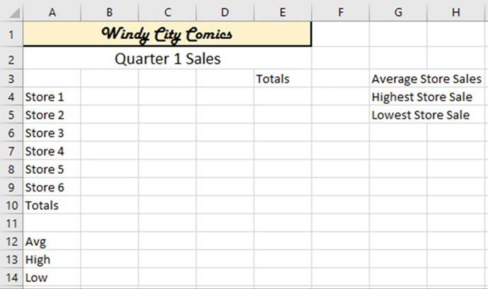
Figure11-45.Makeyourworksheetlooklikethisworksheet.
7.
Select the cell range B3:E3. Bold the text. Select the Center button in the Alignment group.
8.
Select the cell Range B10:D10.
Hold down your Ctrl key while you drag across cells E4 through E9. Apply the lightest green background
color.
406
CHAPTER 11 ■ TRANSFERRING AND DUPLICATING DATA TO OTHER LOCATIONS
9.
Apply a thick outside border to cell A10. Apply the second
lightest green background color.
10.
Select the cell range B3:D3. Apply a thick bottom border.
Your worksheet should now look
like Figure 11-46.
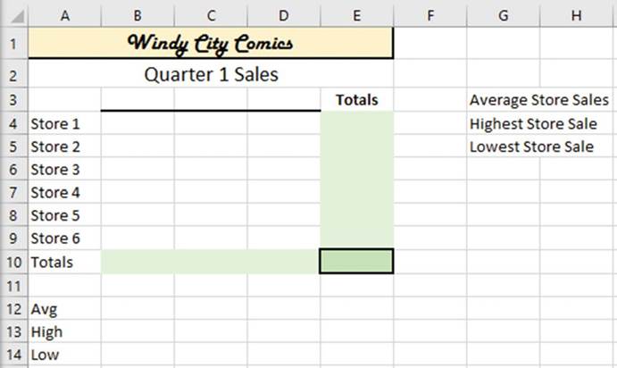
Figure11-46.Yourworksheetshouldnowlooklikethis.
11.
Enter a 1 in cell B4. Use the Autofill
Handle to copy the 1 down through
cell B9. Use the Autofill
Handle in cell B9 to copy the 1 to cell D9.
12.
Select the cell range B4:E10. Click
the AutoSum button.
13.
Enter the formula =Average(B4:B9) in cell B12.
14.
Enter the formula =Max(B4:B9) in cell B13.
15.
Enter the formula =MIN(B4:B9) in cell B14.
16.
Select the cell range B12:B14. Use the Autofill
Handle to copy the formulas through cell D14.
17.
Enter the formula
=Average(E4:E9) in cell I3.
18.
Enter the formula =Max(E4:E9) in cell I4.
19.
Enter the formula =Min(E4:E9) in cell I5.
20.
Select cell range B12:D12. Hold down the Ctrl key and select
cell I3. On the Ribbon�s
Home tab in the Number
group, click the down arrow of the Number Format and select
Number. We are selecting the Number format
so that the averages have two decimal
positions.
407
CHAPTER 11 ■ TRANSFERRING AND DUPLICATING DATA TO OTHER LOCATIONS
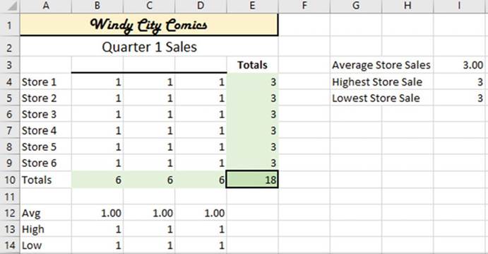
Figure 11-47.Your worksheet should now look like
this worksheet.
Your spreadsheet should now look like Figure 11-47.
21.
Select the cell range B4:D9. Right-click the selection and select Clear Contents. You will get
divide by zero errors
for the Averages because there is no data.
Our template is completed. Now, you need to ungroup
the spreadsheets so that you can enter data into each individual worksheet.
22.
Right-click a selected worksheet and select Ungroup Sheets.
23.
Click each of the worksheets. They
should be identical.
24.
Click the Qtr1 worksheet. Enter
Jan in cell B3, Feb in cell C3, and Mar in cell D3.
25.
Enter any numbers you want to in the cell range B4:D9.
Your
worksheet should look similar to the one in Figure 11-48.
408
CHAPTER 11 ■ TRANSFERRING AND DUPLICATING DATA TO OTHER LOCATIONS
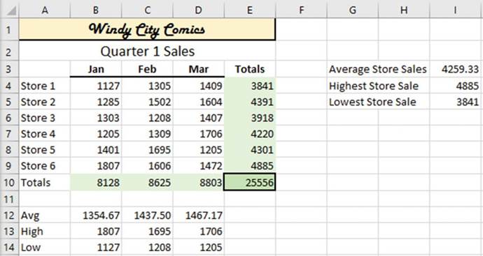
Figure 11-48.Your worksheet should now look like
this worksheet.
26.
Click the Qtr2 worksheet. Change
the heading from Quarter 1 Sales to Quarter 2 Sales. Enter
Apr in cell B3, May in cell C3, and Jun in cell D3.
27.
Enter any numbers you want to in the cell range B4:D9.
Summary
The difference between a
move and a copy is that after you have performed a copy, the data will exist in
both its original location as
well as in the pasted location while a move clears the data from its original
location and stores it in the pasted
location. The Paste Special command has much more capability than just pasting data into a cell. While it is
pasting
it can perform calculations at the same time. It has options for copying only the cell values without
copying
the formatting or copying the formatting without the cell values. The Transpose option for Paste Special
converts row data into column data or column data into row data. The Fill Across Worksheets option copies
data
from one worksheet into multiple worksheets.
Whenever you do a copy, the copy is temporarily stored in the Office Clipboard. You can store 24 items
on the Office Clipboard at a time. This clipboard is shared with other office products so you can easily
copy
and paste between them.
In the next chapter you will see how to convert your data into a table. You can apply multiple sorts and
complex filtering to tables so you can view only the data you want to see and in the order you want to see
it.
409
CHAPTER
12
Working with Tables
A table is a structured
collection of data consisting of a
header row and multiple data rows. A table is used to contain data of a single type such as
orders, sales, inventory, and so on. A table makes it easier to filter, sort, analyze,
summarize, and format your data.
After
reading and working
through this chapter
you should be able to:
�
Create and format a table
�
Sort and filter
a table
�
Add to a table
�
Resize a table
�
Add calculated fields to a table
�
Create slicers
�
Apply themes
�
Apply styles
�
Create conditional formatting
You can pull
data from multiple tables to create another table.
Data in a table can be kept separate from other data in your worksheet. You can
take an existing range of cells and
format them into a table. If you no longer want the data to be in a
table format, you can convert it back to a range.
The last part
of this chapter covers conditional formatting. Conditional formatting improves
the readability of your data by
allowing you to apply formats or
display icons based on cell values. For example, you can have cell data
in a column appear in bold red if the value is less than 0, blue if the value
falls between 0 and 1000, and green if the value is greater than
1000. You can decide how the data will be formatted and create
the rules for those formats.
Creating and Formatting Tables
The process of creating and formatting a table is very simple. Select the data you want to be in a table and
pick a format you would like it to be in. That�s all there is to it.
You format the data you have selected on a worksheet as a table by clicking the Format as Table button.
The Format as Table button
is located on the Home tab in the Styles group. Clicking the Format as Table button brings up a gallery of
styles
for you to select from. See Figure 12-1. The gallery is divided into the categories Light, Medium, and Dark.
Some of the styles have colored column headings; some have cell borders and others do not; some have a
different color for every other row and others do not. If you don�t like any of the styles Excel has
provided
for you then you can create your own style.
411
CHAPTER 12 ■ WORKING WITH TABLES

Format as Table "

Light
 ��������������
 ���������������
 ��������������
 ��������������
 ���������������


---------- ---------- ----- - --- ---
 --------
 -
-


lllllllllm!.11
d


s--


Medium� ----------- ------#---- -----�- =---� �- m-------- .--=--=----
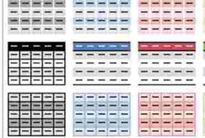
mmmmm mmEE mmEE mmmmE mmmmE mEmmE mmEEE

Dark
jg[TE _


=

Figure 12-1.Gallery of styles. Select the one you want to format your table
412
CHAPTER 12 ■ WORKING WITH TABLES
When you select a style, Excel brings up the Format as Table
dialog box. If you haven�t already
selected the cells
to become a table you can do so at this point.
Be sure the My table has headers check
box is selected if your selected data contains headers.
See Figure 12-2.
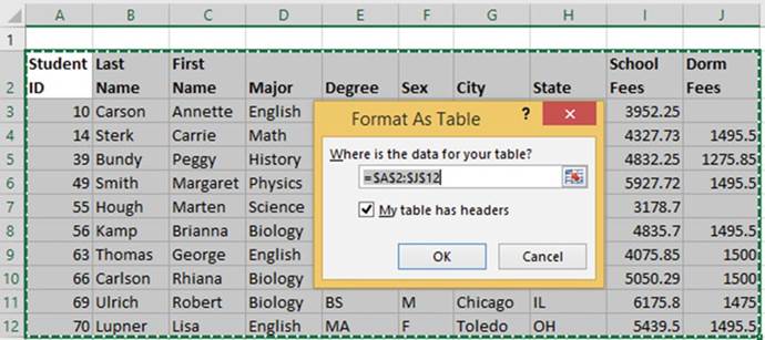
Figure
12-2.Selectthecellsthatyouwanttobecomeatable.Ifyouareincludingheadings,makesureMytablehasheadersisselected
Sort and Filter a Table
Tables display down arrows
to the right of each column header. Clicking one of these down arrows brings up sort and
filter options for that column as illustrated in Figure 12-3.
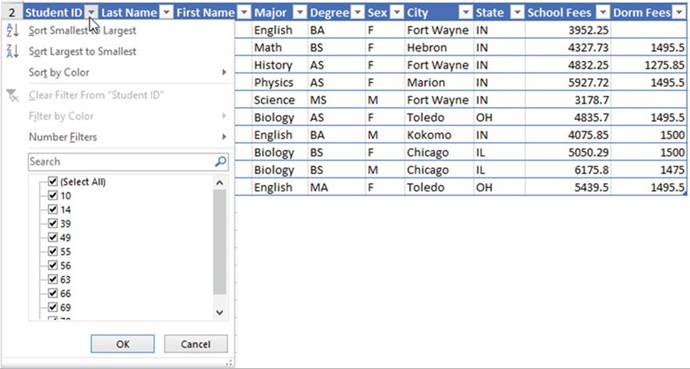
Figure 12-3.Select
down arrow to the right
of the header to select
filters
413
CHAPTER 12 ■ WORKING WITH TABLES
Every unique value that appears in the column is displayed. If there are duplicate values in a column they
are not repeated in the list.
Removing a
check mark in front of a value will prevent the row that contains that value
from being displayed. If you have
removed multiple check marks you can quickly reselect all of them by selecting (Select All). If you only
want to
select a couple of items for filtering, you can deselect (Select All) then just click the
items that you want included in your table.
Filtering does
not rearrange or alter your data; it temporarily hides rows that don't match
the criteria you specify. Removing
filters restores your table to the way it was before the filters were applied.
Columns that have been filtered can easily be identified because the down arrow button changes to a
filtered button
 . Excel displays the applied filter when you hover your cursor over the filtered button.
Adding to the Excel Table
You can add additional
records to the table by typing them in the row after the last record in the
table. After
you press the
Enter key at the end of the record, it will automatically become part of the
table. You can add new
columns in a similar manner by keying a new column to the right of the last
column. You can also expand
the table to include more rows or columns by dragging the table expansion
handle located at the bottom
right-hand corner of the table
 . You can then type
additional data into the expanded area. You can also insert a row or column
anywhere in the table. If you insert a new column, the column heading will be named Column. Double-click the
column heading and change the name to what you want.
. You can then type
additional data into the expanded area. You can also insert a row or column
anywhere in the table. If you insert a new column, the column heading will be named Column. Double-click the
column heading and change the name to what you want.
Automatic expansion of the table can be stopped
by performing the following steps:
1.
Click File ➤ Options.
2.
Click Proofing in the left pane.
3.
Click the AutoCorrect Options
button in the right pane.
4.
Click the AutoFormatasYouTypetab.
5.
Deselect
IncludenewrowsandcolumnsintableAutomaticallyasyouwork.
See Figure 12-4.
6.
Click OK.
7.
Click OK.
414
CHAPTER 12 ■ WORKING WITH TABLES
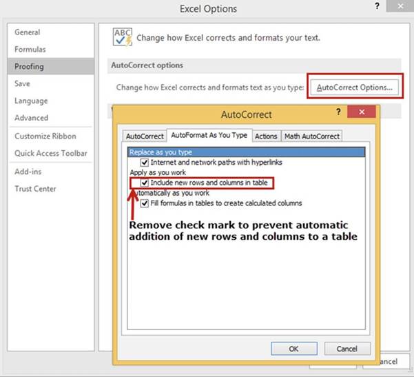
Figure 12-4.Remove check mark from Include new rows
and columns in table
In this exercise you will create a table and
then apply filters to different columns so that you can view only the data that
you want to see.
1.
Open the workbook named Chapter 12. Click the worksheet named �Students.� See
Figure 12-5.
415
CHAPTER 12 ■ WORKING WITH TABLES
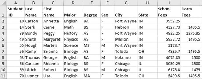
Figure12-5.DataonworksheetStudents
2.
Select the cell range A1:J11.
3.
Click the Home tab on the ribbon.
Click the Format
as Table button
in the Styles group.
4.
Click the first style in the third row of the Medium category. This will be Table
Style Medium 15. See Figure 12-6.
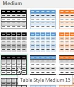
Figure12-6.SelectTableStyleMedium15
5.
Since you have already selected
the range, Excel just wants you to verify it. Since you included your headers in the table,
you need to select My table has headers. See Figure 12-7. Click the OK button
416
CHAPTER 12 ■ WORKING WITH TABLES
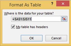
Figure12-7.SelectMytablehasheaders
6.
Click the down arrow to the right of Student
ID. Click Sort Largest
to Smallest. The table is rearranged so that the record with the highest
Student ID appears
first.
See Figure
12-8.
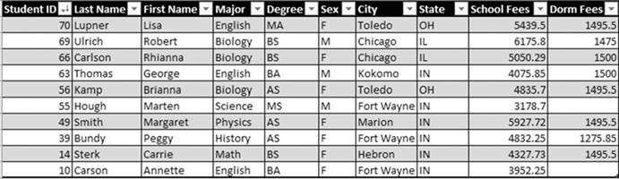
Figure 12-8.Table
has been sorted so that the highest
Student ID appears
first
A down arrow icon has been added to the button to the right of Student ID
(see Figure 12-9). This is to inform you that the column is
sorted from largest to smallest.
7.
Click the down arrow to the right of City. The list displays all the values in the City column.
We have a very small table, but if the column consisted
of thousands of different cities we could use the Search box to find the city we wanted to use.
8.
Click the check box for (Select All)
to deselect all items in the list.
9.
Select the Fort Wayne check box.
10.
Click the OK button. Only the records
that have Fort Wayne for a city are displayed. See Figure 12-9.
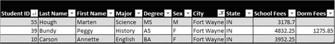
Figure 12-9.The
City column has been filtered
to only show records that have Fort Wayne for a city
417
CHAPTER 12 ■ WORKING WITH TABLES
11.
The button to the right
of City now displays a filter icon so that we can easily see that this column is being filtered. Move your
cursor
over the filter
icon. The tool tip displays
the filter that is being
applied to the column. See Figure 12-10.
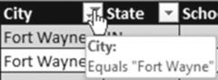
Figure12-10.Movecursoroverfiltericontoviewtooltip
12.
Click the Filter
button to the right of City. A highlighted check
mark appears to the left of the column data.
See Figure 12-11. This is to inform you that the column is being filtered
by one or more of its values.
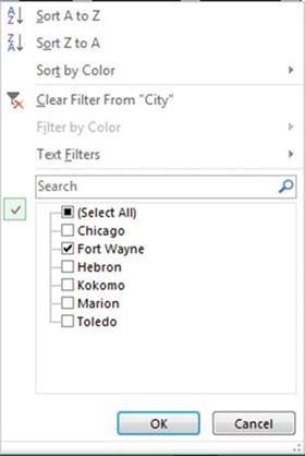
Figure 12-11.Highlighted check mark means
that the field
is currently being
filtered
13.
Click Clear Filter from �City.�
All of the data is now displayed.
14.
Let�s view only the students who are getting a BS degree in Biology:
a.
Click the down arrow to the right
of Major.
b.
Deselect (Select All).
c.
Select only Biology.
d.
Click the OK button.
418
CHAPTER 12 ■ WORKING WITH TABLES
15.
Click the down arrow to the right of Degree.
Select only BS. Click the OK button. Both buttons should have a filter icon on them. Only those
records that meet both conditions are displayed. See Figure 12-12.
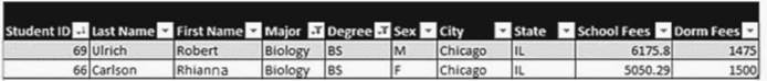
Figure12-12.ResultoffilteringBiologyforMajorandBSforDegree
16.
Click the Filter button to the right of Major. Click Clear Filter from �Major.�
17.
Click the Filter button to the right of Degree. Click Clear Filter from �Degree.�
18.
Let�s find students who have ann in
their first name but not the letters tt:
a.
Click the down arrow to the right of First Name.
b.
Select Text Filters and then
click Custom Filter.
c.
Click the down arrow for the first drop-down box and select contains.
d.
Press the Tab key and enter ann in the next box.
e.
Press the Tab key. Select And.
f.
Click the down arrow in the next box and select does not contain.
g.
Press the Tab key. Enter tt in the box. See
Figure 12-13.
h.
Click the OK button.
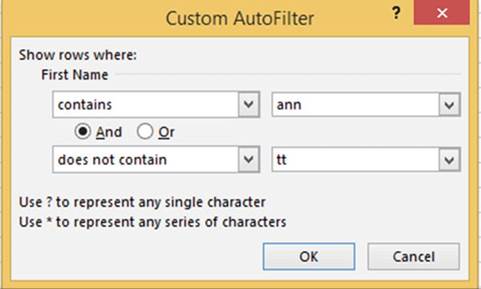
Figure 12-13.Filter
for First Name that contains ann but doesn�t contain the letters tt
Records for Rhianna and
Brianna are displayed because they both contain ann. The record for Annette doesn�t display because even
though the name contains Ann it
also
contains tt.
See
Figure 12-14.
419
CHAPTER 12 ■ WORKING WITH TABLES

Figure12-14.ResultoffilteringFirstName
19.
Move your cursor
over the Filter button to the right of First Name. The tool tip displays the filter that is being applied to
the
column. See Figure 12-15.
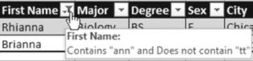
Figure 12-15. Tool tip for filter
20.
Click the Filter button to the right of First Name. Click Clear
Filter from �First Name�.
21.
Let�s find the three students who are paying the most for their school
fees.
a.
Click the down arrow to the right of School Fees.
b.
Select Number Filters.
c.
Click Top 10. You are not limited to the top 10. You can enter however many items you want
displayed. You can select items from the bottom by selecting
Bottom from the first drop-down
box.
d.
Enter the data shown in Figure 12-16.
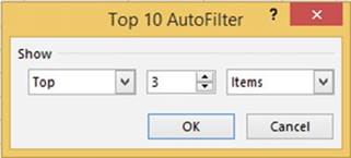
Figure 12-16. Filter for top 3 items.
e.
Click OK. The
result is the top three highest school fees as shown in Figure 12-17.
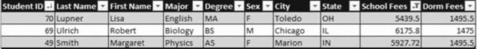
Figure12-17.Filteredfortopthreehighestschoolfees
420
CHAPTER 12 ■ WORKING WITH TABLES
22.
Click the Filter button to the right of School Fees. Click Clear Filter from �School
Fees.�
23.
Let�s find the 30% of the students who are paying the least for their
school fees:
a.
Click the down arrow to the right of School Fees. Select Number Filters.
b.
Click Top 10.
c.
Select Bottom in the first Box. Enter
30 in the middle box. Select
Percent in the third box. See
Figure 12-18.
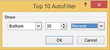
Figure 12-18. Filter for bottom 30%
d.
Click OK. The
result is the bottom 30% of the school fees as shown in Figure 12-19.
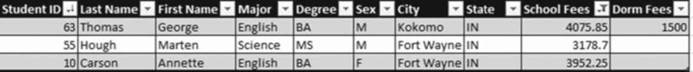
Figure12-19.ResultoffilteringSchoolFeesforbottom30%
24.
Click the Filter
button to the right of School Fees. Click Clear Filter from �School
Fees.�
25.
Let�s find the students who are paying
above average for their school
fees compared to the other students in the table. Click the down arrow
to the right of School Fees. Select
Number Filters. Click Above Average. Figure
12-20 shows the results.
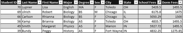
Figure 12-20.Result of selecting Above Average for
School Fees
421
CHAPTER 12 ■ WORKING WITH TABLES
26.
Click the Filter
button to the right of School Fees. Click Clear Filter from �School
Fees.�
27.
Right-Click any cell in the table. Select
Table from the context menu and then
click
Totals
Row.
28.
Click the total in cell J12. Click the down arrow to the right of the
cell. Select
Average.
29.
Click inside cell I12. Click the
down arrow to the right of the cell. Select
Average.
30.
Change the text in cell A12
from Total to Averages. See Figure 12-21.
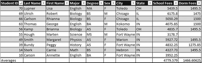
Figure12-21.Resultofchangetoaveraging
You have learned how to filter data from a table by clicking the down arrow to the right of the column head
you want to filter and then selecting only the values you want to view. Next, you will learn an alternative
method of filtering by using a slicer.
Filtering Data with a Slicer
Rather than filtering a table by using
the filter buttons next to the column heads you can create slicers. Slicers
don�t provide all of the options that table filter buttons provide, but they do
make it visually easier to see what has been selected.
In this exercise you will create two slicers to filter a table.
1.
Continue working with workbook Chapter 12 that you used in Exercise 12-1. Click
anywhere within the table.
2.
Click the Design
tab. In the Tools group click the Insert Slicer button. This brings up the Insert
Slicers dialog box. See Figure
12-22.
422
CHAPTER 12 ■ WORKING WITH TABLES
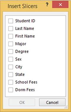
Figure12-22.InsertSlicersdialogbox
3.
Select Major and City. Click
the OK button. See Figure 12-23.
Figure 12-23. Slicers for Major and City
4.
Click Biology in the Major slicer. Excel
only shows the students with a Biology
major. The City slicer highlights Chicago and Toledo
because the Biology
majors are from these two cities.
423
CHAPTER 12 ■ WORKING WITH TABLES
5.
In the Major slicer click the Multi Select button
 �in the upper right corner this allows you to
select more than one item from the slicer.
�in the upper right corner this allows you to
select more than one item from the slicer.
6.
Select Biology and
English. The City slicer now highlights
Chicago, Fort Wayne, Kokomo, and Toledo because this is where
the Biology
and English
majors are from.
7.
Click the Clear Filter button in the upper right-hand corner of the Major
slicer.
8.
In the City slicer click Hebron. The
record for Carrie Sterk appears.
Convert
Table Back to a Range
1.
Convert the Table
back to a range by right-clicking any cell in the table and then selecting Table.
2.
Click Covert to Range.
3.
A message box displays asking
you to confirm that you really do want to convert the table to a range.
Click the Yes button.
All the filter buttons have been
removed from your column headings.
You have
learned how to create a table, sort it, filter it, and then convert it back to
a range. Next, you will learn
how to change the appearance of your workbooks by using existing themes and
creating new ones.
You may want to create custom themes to give your documents or your company�s documents a consistent
appearance.
Using Themes
A theme in Excel consists
of colors, a heading and body font, and graphic effects applied to a worksheet. Themes are
located on the Page Layout tab in the Themes group. See Figure 12-24. You can also create your own themes.
You can use themes to
enhance the look of your spreadsheets as well as to give them a
consistent look. You could, for instance, apply different themes to different projects, or maybe your company
elects to always use the same theme. Microsoft Word and PowerPoint have the same themes available as those
found in Excel.
424
CHAPTER 12 ■ WORKING WITH TABLES
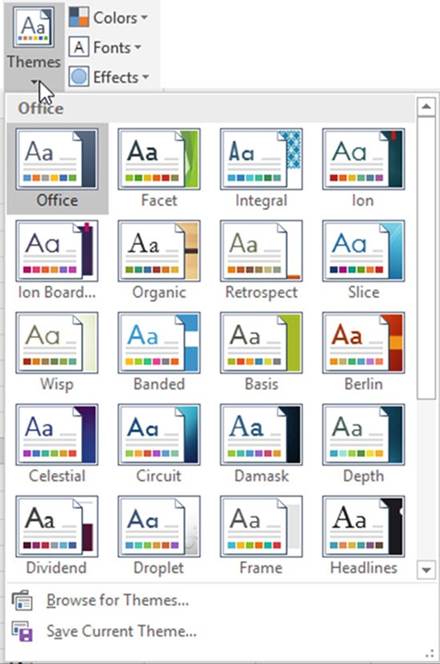
Figure 12-24. Themes gallery
Office is the Default
theme.
425
CHAPTER 12 ■ WORKING WITH TABLES
If you click the down arrow for Font on the Home Tab�s Font Group you will see the two theme fonts
above all of the other fonts. See Figure 12-25.
Figure12-25.TheThemefontsareCalibriLightandCalibri
In this exercise
you will using
existing themes to change the appearance of a workbook. You will also create your own custom
theme.
1.
Open the Chapter 12 workbook. Select
the Theme Practice worksheet.
2.
Click the Ribbon�s Page Layout tab.
3.
In the Themes
group click the Theme�s button.
Move your cursor across the different themes as you notice each one�s effect.
4.
Click the ribbon�s Home tab. In the Font group notice that the font is Calibri with a size of 11.
5.
Click the down arrow for the fill color and observe what colors are
available
6.
Click the down arrow for the font color and observe what colors are
available
7.
Click the Ribbon�s Page Layout tab.
8.
In the Themes group click the Theme button. Click the Savon theme.
9.
Click the Ribbon�s Home tab. Notice
that the default font is now Century Goth size
11. Click the down arrow
for fill color.
Notice that the theme colors
have changed. Click
the down arrow
for the font color. The theme colors
have changed here as well.
10.
Click the Ribbon�s
Page Layout tab. Click
the Theme button. Select Office.
11.
A theme consists
of colors, fonts,
and effects. If you didn�t
want to change
an entire theme you can change part of it, such as just changing
the colors. In the Themes
group click the Theme color button. Select
Grayscale.
426
CHAPTER 12 ■ WORKING WITH TABLES
12.
Click the ribbon�s
Home tab. You still have the Office
Theme�s default font of Calibri,
but if you look at the colors available from the color fill or the font color they will be from the
grayscale palette.
13.
Click the Ribbon�s Page Layout tab. Click
the Theme colors button.
14.
Click
Customize Colors. The Create New Theme Colors window displays where you can select the colors you want to
use for your customized
colors. See Figure 12-26. After you have selected some colors, enter a name. Use your name followed by
CustomColors. Click the Save button.
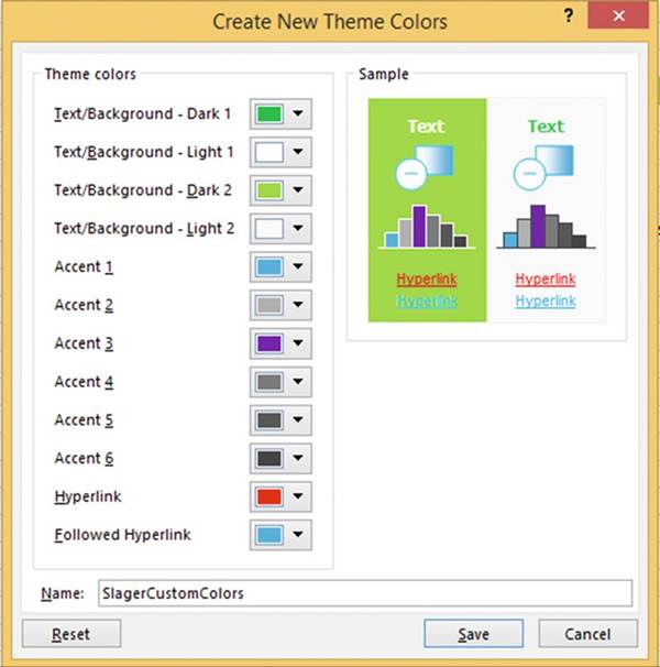
Figure 12-26. Theme Color options
15.
Click the Theme
colors button. Your custom colors
should appear at the top. See Figure
12-27.
427
CHAPTER 12 ■ WORKING WITH TABLES
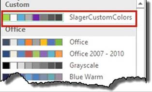
Figure 12-27.The theme colors you selected appear at
the top under Custom
You can do
the same
thing for
Theme Fonts; either select
a font
or create
a Custom
Font. You
can select
a Theme effect but you can�t
create a custom one. Figure
12-28
shows the Theme Effects gallery
for the
default Office Theme. Effects provide
subtle differences like a slightly
different edge to your Shapes,
SmartArt, Images, Charts, Tables, and
WordArt.
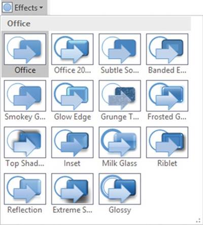
Figure12-28.ThemeEffectsfortheOfficeTheme
428
CHAPTER 12 ■ WORKING WITH TABLES
16.
Click the Themes
button. Click Save Current Theme.
Enter a
name for
your theme
and click
the Save
button. The theme you saved contains
whatever is currently selected in
Theme Colors,
Theme Fonts, and Theme
Effects.
17.
Click the Theme
button. Your theme
should appear in the Custom
group at the top as shown in Figure 12-29.
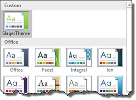
Figure 12-29.The
theme you created
appears above the other themes
in the Theme Gallery
18.
Click the Office theme.
You
have seen how to apply formatting through
a theme. Next,
you will learn how apply
styles to cells.
Applying and Defining Cell Styles
Cell styles provide a way
of improving the look and readability of your spreadsheet. Figure 12-30 shows the cell styles. They can be
accessed from
the Home tab�s Styles group by clicking the Cell Styles button. The Cell Styles are divided into five
categories:
�
Good, Bad, and Neutral
�
Date and Model
�
Titles and Headings
�
Themed Cell Styles
�
Number Format
429
CHAPTER 12 ■ WORKING WITH TABLES
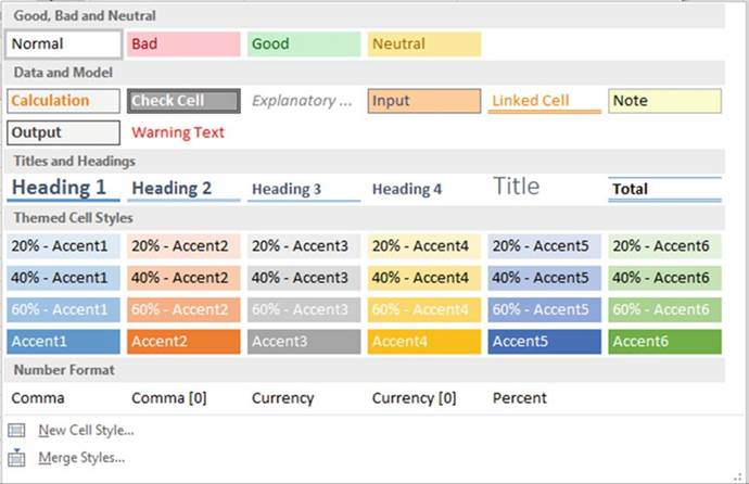
Figure 12-30. Cell styles
Styles provide you with an easy way to give a consistent
format to certain cells, such as those that contain what the company would
consider good news and those that contain what the company would consider bad news, cells that are used
for Input and those that are used for output, those cells that contain links, and so on. You can also use
Themed Cell Styles, which provide different amounts of transparency using the same color. These
predefined styles are located at Home ➤ Styles ➤ Cell
Styles. Themed Cell Styles are derived from the theme you are currently using. If you change your
document theme, your themed cell styles will be different. You apply styles to your worksheet by first
selecting those cells you want to apply the style to and then clicking the
appropriate style from the Cell Styles gallery. A nice feature of the styles is
that you can see exactly how a
style will affect your spreadsheet before you ever apply it. Move your mouse
over any style to get a visual
preview of how it will affect your spreadsheet.
Maybe there is no style in the Cell Style gallery that meets your needs.
No problem; just create your own style. To do this, click New Cell Style� at the bottom of the
Cell
Styles gallery. This brings up the Style dialog box where you can assign a name to
your new style.
Styles can be deleted by displaying the Cell Styles gallery, right-clicking the style, and then pressing the
Delete key.
430
CHAPTER 12 ■ WORKING WITH TABLES
In this exercise you will apply existing cell styles and then you will
create a new cell style and apply it.
1.
Open Workbook Chapter 12. Click the Cell Styles worksheet tab.
2.
Click cell A1. On
the ribbon�s Home tab, in the
Styles group, click on
the More down arrow to the right
of Cell Styles.
3.
Under the Titles and Headings
group, Click Heading 1.
4.
Select cells A3:J3. Click the down arrow for Cell Styles. Select 20% -Accent 5.
5.
Select cells I14:J14. Click
Cell Styles. Select Total.
6.
Select cell J8. Click Cell Styles. Select Bad.
Create a
new Style
1.
Click Cell Styles. Click New Cell Style.
2.
Click the Format button.
3.
Select the Alignment tab. Make the text 45 degrees.
4.
Select the Border tab. Select a
light blue color. Select Outline in
the Presets.
5.
Select the Fill tab. Select a light gold color.
6.
Click the OK button.
7.
Change the style name on the Style window to your last name
followed by Style, for example �SlagerStyle.�
8.
Click the OK button.
9.
Select cells A3:J3.
Click Cell Styles.
The style you created should
be in the Custom group.
See Figure 12-31.
Figure12-31.StyleyoucreatedshouldbeintheCustomgroup
431
CHAPTER 12 ■ WORKING WITH TABLES
10.
Click the style you created. See
Figure 12-32.
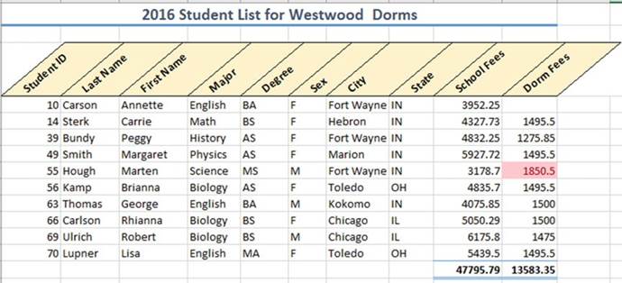
Figure12-32.Formattedwiththestyleyoucreated
You have learned how to apply consistent formatting by using themes and cell styles. Next, you will learn
how to format based on a condition (e.g., applying a format to all cells in a column that have a value over
500).
Conditional Formatting
Conditional formatting
formats cells based on the values they contain. The formatting is conditional
based on criteria that you
determine. Cells that are of special interest to you can be highlighted. You
can apply conditional formatting to
tables or any range of data.
If you have a large amount of data in your spreadsheet it can make those cells of importance stand out,
or it can give you a quick visual overview about the range of the values in a column.
In this example you will create formatting
based on whether certain conditions are met.
You will learn how to edit, delete,
and create new formatting rules.
1.
Open Workbook Chapter
12.
2.
Click the Orders tab. Figure 12-33 shows the data.
432
CHAPTER 12 ■ WORKING WITH TABLES
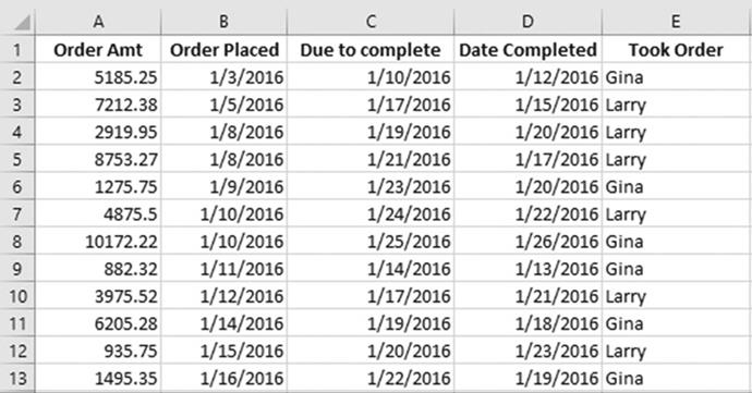
Figure 12-33. Data on the Orders tab
Top/Bottom
Rules
1.
Select the cell range A2:A13
2.
On the Home tab in the Styles group click Conditional Formatting.
3.
Select Top/Bottom Rules.
4.
Select Top 10%. You are not limited
to the Top 10%. You can enter any value. Change 10 to 25 to get the top 25%.
The top 25% will be highlighted with whatever
formatting you select. It is
currently showing with Light Red Fill
with Dark Red Text.
Click the down arrow and then click each option as you observe how it affects
the selected range.
Keep repeating this until you have seen the effect of each option. Finally,
click Custom Format.
This brings up the Format Cells window. You can make selections from any of the tabs.
5.
Click the Font tab. Select
Bold. Click the down arrow
for color. Select
Purple. Click the Border tab. Select Outline.
6.
Click the OK button. Figure 12-34 shows the results.
433
CHAPTER 12 ■ WORKING WITH TABLES
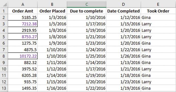
Figure12-34.Formattedwithtop/bottomrules
Clear
Rules
Next, you will clear the rules you set for cell
range A2:A13
1.
With the cell range still selected, click
Conditional Formatting, select
Clear Rules then select Clear Rules from Selected Cells. See Figure 12-35.
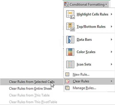
Figure12-35.SelectClearRulesfromSelectedCells
434
CHAPTER 12 ■ WORKING WITH TABLES
2.
With cell range A2:A13 still selected, select Conditional
Formatting then select Top/ Bottom Rules then select Below Average. Leave the format as Light Red Fill
with Dark Red Text.
3.
Click the OK button. The smaller values should be highlighted. Click
a blank cell so that you can see the results.
4.
Let�s clear the rules again. The only rules we currently have for this worksheet are those for the
cell range A2:A13.
Click Conditional Formatting, then select Clear Rules, and then select
Clear Rules from Entire Sheet.
Highlight
with Data Bars
1.
Select the cell range A2:A13,
select Conditional Formatting, and then select
Data Bars.
2.
Move your cursor over each of the Gradient Fill and Solid Fill Colors. See Figure 12-36.
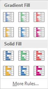
Figure12-36.ConditionalFormattingDataBars
The larger the value in the cell, the longer the data bar will be. See Figure 12-37.
Don�t Select any.
■
Note� Some of the conditional formats have more of an impact if the column
widths are wider.
435
CHAPTER 12 ■ WORKING WITH TABLES
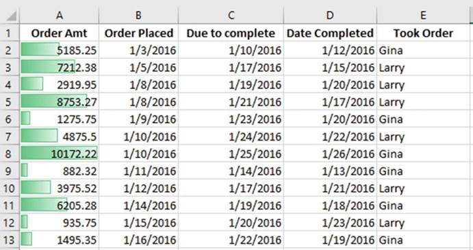
Figure12-37.Thelargerthevalueinthecellthelongerthedatabar
3.
With cell range A2:A13 still selected, select Conditional
Formatting ➤ Highlight
Cells Rules ➤ Greater
than. Enter
5000 in the text box and select Yellow Fill with Dark Yellow Text. See Figure 12-38.
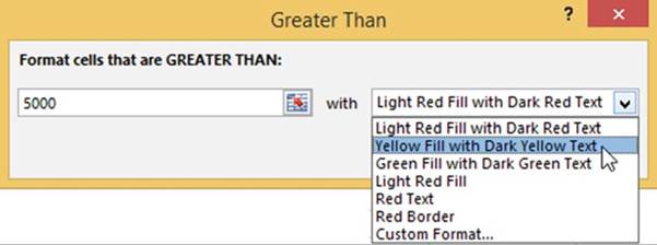
Figure 12-38. Conditional formatting
4.
All values in the range that are greater than 5000 should
be highlighted. Click the OK button.
Highlight
Duplicate or Unique Values
1.
Select the cell range B2:B13.
2.
Select Conditional Formatting ➤ Highlight Cell Rules ➤ Duplicate Values.
436
CHAPTER 12 ■ WORKING WITH TABLES
3.
You can highlight duplicate cells or you can highlight those
that don�t have a duplicate
by selecting Unique.
See Figure 12-39. Select
Duplicate.
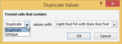
Figure12-39.FormattingforDuplicateValues
4.
Click the OK button.
Highlight
Values Between Other Values
1.
Select the cell range C2:C13.
2.
Select Conditional Formatting ➤ Highlight Cell Rules ➤ Between.
3.
Enter 1/15/2016 for the first date and enter 1/19/2016 for
the second date. Click the down
arrow for the format and then select Custom Format.
4.
Click the Font tab and then select Bold for the Font style.
5.
Click the Fill tab and then select a light green color.
6.
Click the OK button for the Format Cells dialog box.
7.
Click the OK button for the Between dialog box.
Highlight
Values Greater Than Another Value in Another Column
We want to
highlight the dates where we didn�t complete an order by its due date.
1.
Select cell range D2.
2.
Select Conditional Formatting ➤ Highlight Cell Rules ➤ Greater Than.
3.
With the date from D2 currently highlighted in the Greater
Than window, click Cell C2. The text box displays
the cell address
in absolute form. We will need to copy the formatting so select the text and change it to =C2. See Figure
12-40.
437
CHAPTER 12 ■ WORKING WITH TABLES
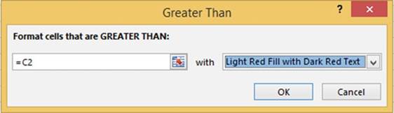
Figure12-40.HighlightvaluesthataregreaterthanthoseincellC2
4.
Click the OK button.
5.
Drag the Autofill
Handle from D2 down through
D13. Click on the Autofill
options button below
the selected data.
Select Fill Formatting Only.
Highlight
Specified Text
1.
Select cell range E2:E13.
2.
Select Conditional Formatting ➤ Highlight
Cell Rules ➤ Text that Contains. Leave Gina in the first text box. Click the down arrow for the
format then select Red Text.
3.
Click the OK button.
Edit,
Delete, and Create New Rules
1.
Click Conditional Formatting and then select Manage Rules.
2.
Click the down arrow for Show formatting rules for and then select This Worksheet.
3.
Select the Rule for Cell Value contains �Gina� and then click the Edit
Rule button.
You
have more options here to work with. Select beginning
with. See
Figure 12-41.
438
CHAPTER 12 ■ WORKING WITH TABLES
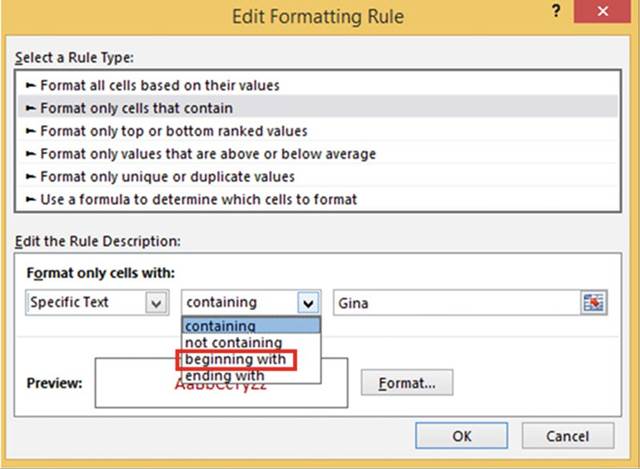
Figure 12-41. Select beginning with
4.
Change Gina to just G. (Now anybody whose name starts with G will
be highlighted.)
5.
Click the Format button.
6.
Click the Font tab. Select Bold
Italic from the Font style.
7.
Click the OK button for Format Cells.
8.
Click the OK button for the Editing Formatting Rule dialog box.
9.
Click the OK button for the Conditional Formatting Rules Manger dialog
box.
10.
Change the name Larry in cell E3 to Gary.
It should now be highlighted because it starts with a G.
439
CHAPTER 12 ■ WORKING WITH TABLES
Applying
Conditional Formatting to a Table
You applied conditional formatting but what if you added additional rows of data?
The conditional formatting will apply to those cells
immediately below the selected rule range except
for dates. For date columns
use the Autofill
handle to copy and then click on the Autofill
options button and select Fill Formatting Only.
1.
Add an additional row of data that meets the conditional
rules for each column. See row 14 in Figure 12-42.
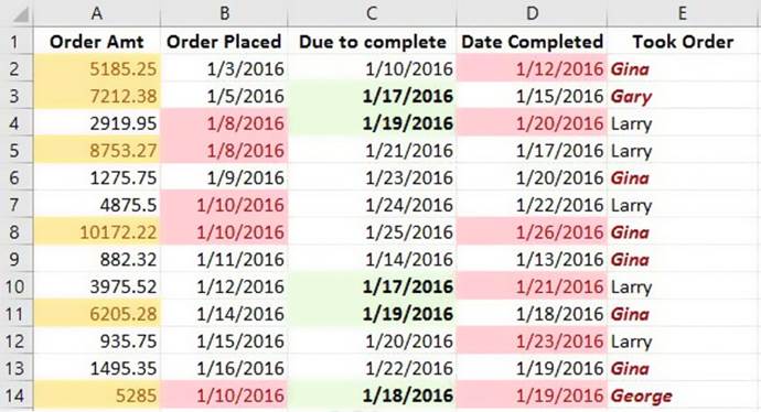
Figure12-42.Resultofaddinganadditionalrow
2.
Click the Lab Scores worksheet tab.
3.
Select cell range B2:B8.
4.
Select Conditional Formatting ➤ Color Scales. Move your cursor
over each option
to see how affects the cell background colors.
440
CHAPTER 12 ■ WORKING WITH TABLES
5.
Select one and click the OK button.
We want to highlight the student averages
based on their scores. The grade
scale is as follows:
90�100 A
80�89 B
70�79 C
60�69 D
0�59 F
6.
Select the cell range F2:F8.
7.
Click Conditional Formatting and then select Icon Sets. Select the first option in the Indicators
group.
See Figure 12-43.
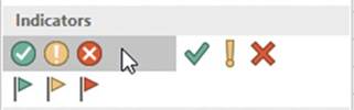
Figure12-43.IndicatorsgroupintheIconSets
We want to use an icon with a green
circle and a check mark in it for those
who have an A or a B, a yellow
circle icon with an exclamation mark in it for students
who have a C, and a red circle with an X through it for those
students who have a D or an F.
8.
Click Conditional Formatting and then select Manage Rules.
9.
Click the Icon Set and then click the Edit Rule Button.
You don�t have to use all of the icons from
one set you can pick amongst the different
icons. See Figure 12-44.
441
CHAPTER 12 ■ WORKING WITH TABLES
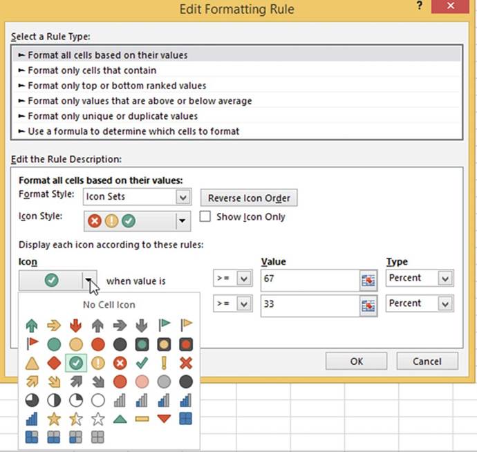
Figure 12-44. Select an icon
10.
Change the Type for the green and yellow icon to Number.
The greater than or equal to sign is already
selected. Enter .8 for the green icon Value.
442
CHAPTER 12 ■ WORKING WITH TABLES
11.
Enter .7 for the value for the yellow icon. the greater
than or equal to sign should already
be selected. The type should be Number.
The red icon should show that it will display
for any value less than .7. See Figure 12-45.
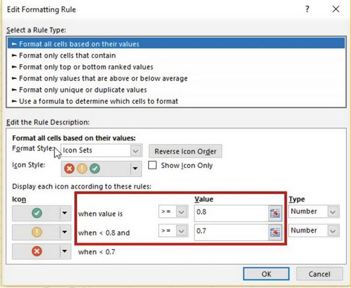
Figure 12-45. Formatting rule
12.
Click OK. Figure 12-46 shows the results.
443
CHAPTER 12 ■ WORKING WITH TABLES
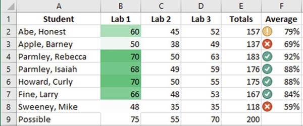
Figure12-46.Resultofapplyingformattingrule
13.
Change Cell D7 from 53 to 44. Your
icon should change to the yellow icon.
Summary
A theme in Excel consists
of colors, a heading and body font, and graphic effects applied to a worksheet.
You can also create your own
themes. You can use themes to enhance the look of your spreadsheets as well as
to give them a consistent
look. You could, for instance, apply different themes to different projects, or
maybe your company elects to
always use the same theme. Microsoft Word and PowerPoint have the same themes available as those found in
Excel.
Microsoft
Office Themes consists of galleries of colors, heading and body fonts, and
graphic effects. You
can click the various themes and at the same time view how they affect your
worksheet. You can select the one that is most pleasing to you, or perhaps your company requires a
particular theme so
that all of its documents
have a consistent look. If you can�t find a theme that matches your needs, you
can create your own by
making selections from the color, heading and body font, and graphic effect
galleries.
Rather than
manually formatting your cells, you select from groups of predesigned cell
styles. The groups are Good, Bad, and
Neutral; Data and Model; Titles and Headings; and Number Format. Like themes, cell styles
can give your worksheets a consistent look, such as always giving your
headings, titles, and totals the same appearance.
You can convert the data in your worksheet
to a table and then convert it back again to its original format. You create a table by selecting the data
you want to convert into a table and then clicking the Format as Table button located in the Ribbon�s
Styles group. Converting data to a table allows you to filter data by clicking the drop-down arrow to the
right of a column head. You can then either select the values that you want
to use for your filter or create a custom filter; if the data is text, you can select a Text Filter and if
the data is Numeric, you can select a Numeric
Filter. Another way of filtering
table data is to create slicers. Slicers
let you see exactly what is being filtered without
having to look into the table filters.
You can format
cells with a variety of colors or icons to highlight cells that are of
particular interest. For example, you could highlight cells whose value is in the top 20% with one
icon, a value within the middle 60% with another icon, and a value in the bottom 20% with yet another
icon.
The next
chapter covers charts. Excel makes it very simple to take your spreadsheet data
and turn it into a chart. Charts make it easy to find trends in your
data that you might not otherwise detect.
444
CHAPTER
13
Working with Charts
Where would we be without
charts? Not only are charts more appealing
to our eye than raw data, but they also make it much simpler
for us to spot trends.
The old saying �a picture
is worth a thousand words� also applies to charts.
Managers don�t always want to look at every record in a spreadsheet; they would rather make their decisions
based on trends,
whether they be good or bad. By looking at trends, management can decide what actions the company should
take in the future.
Charts can summarize vast amounts of data and also show relationships between
data. Charts make it easier to see such things as what lines of product are more profitable, what the most
profitable time of year is, whether
the profitability of the company
is on the rise or going down, what departments are doing well and which are not, and on and on.
After reading and
working through this chapter you should be able to:
�
Use shortcut keys to create charts
�
Change chart types
�
Add a data point
�
Change the data source
�
Create a pie chart
�
Create a pie of a pie chart
�
Crate a pie of a bar chart
�
Create a chart with multiple
data chart types (Combination Chart)
�
Create a Treemap chart
�
Create a Sunburst chart
Chart Types
Excel provides a wide variety
of chart types
to choose from to best display your data. What type of chart you should use depends upon the data you are
charting. Before
creating a chart
you need to decide what it is you want the chart
to say. Once you have a chart
selected you can change the format of the entire
chart by changing its theme, or you can change the individual components of the chart.
Excel provides a wide variety of different chart options.
As you will see later,
Excel looks at the data you have selected, makes
a quick analysis
of it, and then provides recommended chart types for your data.
The Ribbon�s Insert
tab in the Charts group
displays the available chart types. Clicking
a down arrow next to one of the chart types
will display available variations of that chart type.
See Figure 13-1.
445
CHAPTER 13 ■ WORKING WITH CHARTS
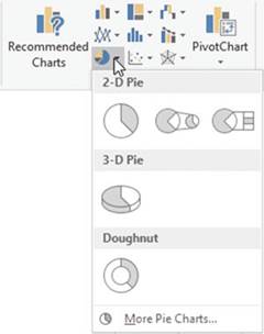
Figure 13-1. Variations of the pie chart
Clicking the Charts group
dialog box launcher
as shown in Figure 13-2 brings up the Insert Chart
dialog box (Figure 13-3).
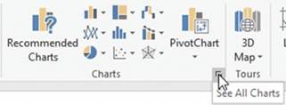
Figure 13-2. Charts group
The Insert
Chart dialog box has two tabs. The Recommended Charts
tab displays the Recommended Charts
for the data you currently have selected in your worksheet. See Figure 13-3. The charts displayed here are
using
the data that you have selected. Clicking
a chart type gives a description of what that chart type can be used for.
446
CHAPTER 13 ■ WORKING WITH CHARTS
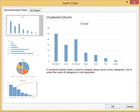
Figure 13-3.Insert Chart dialog box with
Recommended Charts tab selected
The Recommended Charts are just a suggestion. You don�t have to use Excel�s suggestion. The All Charts tab
shows all of the chart types in the left pane. Clicking
a chart type in the left pane will display
all of the variations of that type in the right pane. See Figure
13-4. The charts displayed here are using the data you currently
have selected on your worksheet. In the left pane there is an option to view your most recent chart.
447
CHAPTER 13 ■ WORKING WITH CHARTS
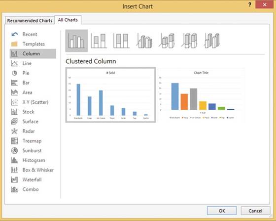
Figure13-4.VariationsfortheColumnchart
Creating and Modifying
Charts
There are several ways to create a chart, including using the options
on the Insert tab shown in the preceding section.
The easiest way to create a default
2D Clustered bar chart is by selecting
the data you want to display in your chart and then
�
Pressing the Alt + F1 key if you want to display the chart on the same worksheet as the data,
or
�
Pressing F11 if you want the chart to appear
on a separate worksheet.
Once you have created
your chart you can change
it in so many ways.
Some of the changes you can make are the following: the type of the chart,
its location, its style, what is displayed in the chart,
reversing the
columns and rows, adding or removing
items from the chart, changing
the color and appearance of individual bars, and adding or removing
legends, titles, data tables, the incremented value on the plot area, and so on.
Selecting the chart adds two contextual tabs to the Ribbon. The contextual tabs Design and Format
appear under the heading Chart Tools. The Design tab is mostly used for making changes
that affect the entire chart while the Layout tab is used for changing
the look of individual elements
in the chart.
■
Note� Don�t get carried away with trying to make
your charts too fancy and overdoing colors, and so on. The most important thing is how well your chart
conveys the information that you want it to and how easy it is
for the intended audience to read and understand. The audience should be able quickly grasp what the chart
is conveying.
448
CHAPTER 13 ■ WORKING WITH CHARTS
In this exercise you will create and modify column and bar charts from
existing Game Sales data.
1.
Open workbook Chapter 13. Click the Game
Sales tab. Figure 13-5 shows the data.
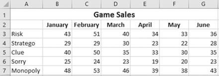
Figure 13-5. Data on Game Sales tab
2.
Select the cell range A2:G7. Press Alt + F1.
Your chart is in a moveable frame.
Move your cursor on the chart frame.
Your cursor should display as four arrows
 .
.
3.
Drag and drop the chart to whatever location you want.
4.
Increase the size of the chart by placing your cursor on the bottom
right of the chart frame
and then hold down the Shift key while you drag the cursor toward
the bottom right.
Holding down the Shift
key makes the chart retain
the same width-to- length ratio.
When a chart is selected,
Excel displays two new tabs on the ribbon: Design
and Format. The two tabs are under the Chart Tools grouping.
■
NoteA chart
consists of many different individual elements. What the elements are depends upon the type of chart
and the data being charted.
On the Ribbon,
click the Format
tab. In the Current Selection group, the Chart
Elements drop-down box displays the current item selected in the chart.
5.
Click the down arrow of the Chart Elements drop-down box. See Figure 13-6.
449
CHAPTER 13 ■ WORKING WITH CHARTS
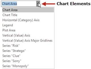
Figure13-6.ChartElementsdrop-downbox
Selecting an item from the Chart Elements list will select that item on
the chart.
6.
Select Plot Area from the Chart Elements
list. The Plot Area is now selected
on the chart.
7.
Select Horizontal (Category) Axis from the Chart Elements
list. The Months
on the Chart are now selected.
Selecting an item from the Chart Elements
list will select that item on the chart and vice versa.
8.
Click the Chart Title on the Chart.
Look at the Chart Elements
drop-down box. It shows that Chart Title is selected.
9.
Drag across the Chart Title text
on the chart to select it. Type Game Sales.
10.
Drag across Game Sales to select it. Right-click Game Sales and then select
Font. Change the font size to 18. Click the OK button.
11.
On the Ribbon�s Format tab, in
the Current Selection group, click Format Selection.
Clicking Format Selection formats the object selected
in the Chart Elements drop- down Box. Since Chart Title is the current
object, clicking Format Selection brings
up the options for formatting the Chart Title:
�
The Title Options menu has options
that affect the area inside
the Chart Title area but outside the text itself.
See Figure 13-7.
�
The Text Options menu has options
that affect only the text.
450
CHAPTER 13 ■ WORKING WITH CHARTS
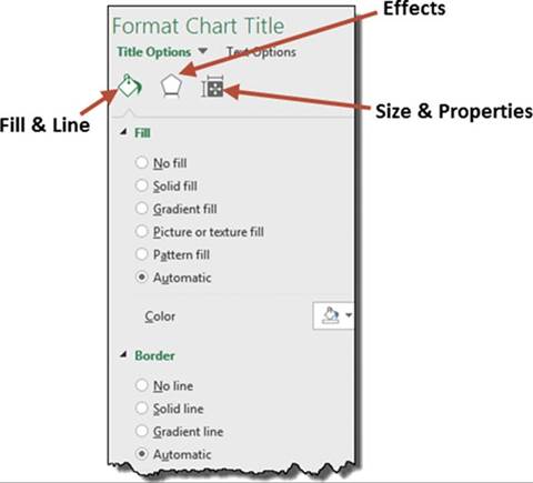
Figure 13-7. Chart options
12.
Click the Fill & Line paint bucket.
13.
Expand the Fill if it isn�t already.
Click Solid fill. Clicking Solid fill brings up options
for Color and Transparency.
14.
Pick the color Orange, Accent
2, Lighter 60% from the Color option.
See Figure 13-8.
15.
Change the Transparency to 50%.
Figure 13-8.Select Orange, Accent2, Lighter 60%
from the Theme Colors
451
CHAPTER 13 ■ WORKING WITH CHARTS
16.
Collapse the Fill. Expand
the Border if it isn�t already.
Selecting an option
other than No line brings up numerous options.
17.
Select Solid line. Change the
color of the border to red.
18.
Increase the size of the border around the Chart Title by changing the width to 2.5.
19.
Change the border to a double line by changing
the Compound Type to Double.
20.
Make the border line corners rounded by changing the Join type to Round.
21.
Click the Effects
button
 . There are four basic effects: Shadow,
Glow, Soft Edges,
and 3-D format.
. There are four basic effects: Shadow,
Glow, Soft Edges,
and 3-D format.
22.
Expand the 3-D Format options.
23.
Click the down arrow for Top
bevel. Select the Cool Slant bevel. See Figure 13-9.
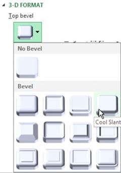
Figure 13-9. Select Cool Slant
The chart title should now appear with a 3-D appearance.

Figure13-10.Thecharttitlenowhasa3-Dappearance
24.
Collapse the 3-D Format options.
452
CHAPTER 13 ■ WORKING WITH CHARTS
25.
Expand the Shadow options. Creating
a Shadow can make an object appear to come off the page:
a.
Click the down arrow for Presets.
b.
There are three groups; Outer, Inner, and Perspective. Click the first option in the first row
(Offset
Diagonal Bottom Right)
c.
Drag the Distance slider to 21 pt.
d.
Drag the blur slider to 16 pt.
26.
Click the Size & Properties button
 .
.
27.
Click the down arrow for Custom angle until the angle is -3.
28.
Drag the Game Sales chart title to the left side of the chart.
29.
Click Text Options. See Figure 13-11.
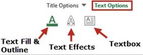
Figure 13-11. Text options
30.
Click Text Fill & Outline
and complete the following steps:
a.
Expand the Text Fill Options.
b.
Select Pattern Fill.
c.
Change the Foreground color to Dark Red.
d.
Change the Background color to Black.
e.
Select the last pattern in the last row (Solid Diamond). See Figure 13-12.
453
CHAPTER 13 ■ WORKING WITH CHARTS
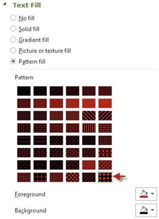
Figure 13-12. Pattern Fill options
31.
On the Ribbon�s
Format tab, in the Current
Selection group, click the down arrow for Chart Elements
and then select Chart Area.
32.
In the Current Selection group, click
the Format Selection button.
33.
In the Format Chart Area pane, select Gradient fill. See Figure 13-13.
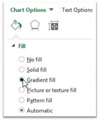
Figure 13-13. Select Gradient fill
454
CHAPTER 13 ■ WORKING WITH CHARTS
34.
Click the down arrow for the Preset
gradients.
35.
Select Light Gradient � Accent 2. See Figure 13-14.
Figure13-14.SelectLightGradient�Accent2
Figure 13-15 shows the result.
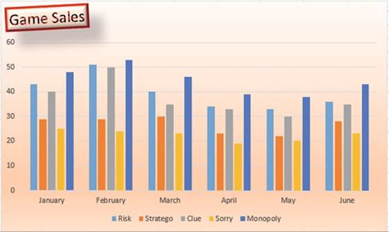
Figure13-15.YourChartshouldnowlooklikethis
36.
Close the Format Selection pane by clicking the X in the
upper right corner of the pane.
37.
Select Legend from the Chart Elements drop-down
box. A border appears around
the legend at the bottom
of the chart. You can move the legend by dragging its border or you can resize it by using
its handles.
455
CHAPTER 13 ■ WORKING WITH CHARTS
Applying
Chart Styles
1.
On the Ribbon under the Chart Tools grouping there is
a Design tab and a Format
Tab. Click the Design Tab.
Excel has a series of predefined styles
that you can select from.
The style buttons
reflect the type of the current chart.
Since we are using a bar chart,
the style buttons
display styles for bar charts.
See Figure 13-16. While
working on a pie chart,
the style buttons
would display pie charts.
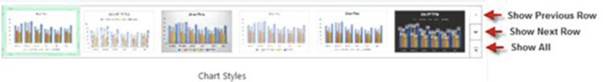
Figure 13-16. Bar
charts
2.
In the Chart Layouts group click the More button (Show All). See
Figure 13-17.
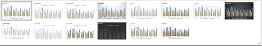
Figure13-17.ChartsavailableafterclickingtheMorebutton
The number of available predefined layouts varies for the different types
of charts.
3.
Move your mouse over the style buttons while noticing how
it changes your chart. A tool tip
displays the name assigned to each button such as Style 1, Style 2, and so on.
4.
Click the Style 6 button. This style adds the individual values to
each bar.
When the chart is selected you will see three
buttons to the right of it. See
Figure 13-18.
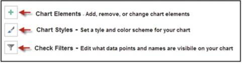
Figure 13-18.These
three buttons display
to tye right of the chart when it is selected
If you click anywhere off the chart these three buttons will not display.
456
CHAPTER 13 ■ WORKING WITH CHARTS
5.
Click the Chart Elements button. See Figure 13-19.
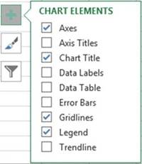
Figure13-19.OptionsforChartElementsbutton
6.
Select Data Labels.
The Data Labels
values appears above
each column.
7.
Select Data Table. The
Data
Table displays the individual values
in a
spreadsheet form. These are the
same values
that are
being displayed
by the
Data Labels
above the
column. Eliminate the Data
Labels by removing the check
mark in
front of
it.
Changing
the Chart Style
1.
Click the Chart Styles button.
What appears here depends upon what you have in your current
chart. Since we currently have a data table in our chart,
all of the charts being presented here have a Data Table.
2.
Move your cursor
over each of the charts
as you scroll through them to see how each option will affect your chart. These
are the same styles that appear on the Ribbon�s
Data Tab in the Chart
Styles group.
3.
Click Style 14. Figure 13-20 shows the results.
457
CHAPTER 13 ■ WORKING WITH CHARTS
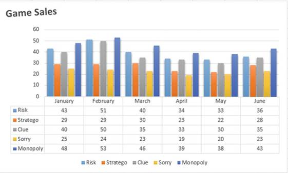
Figure13-20.ResultsafterselectingStyle14
4.
Click the Chart Elements button. Move your cursor over the options. Notice that there is an arrow
to the right of each of the Chart Elements. Clicking the arrow allows you to choose various options for that
Element. The Axis Titles and the Data Labels are not currently selected. Moving your cursor over any
unselected item will show what that item will look like on your chart. Move your cursor over the Axis Title.
There is a horizontal Axis Title and a vertical Axis Title. See Figure 13-21.
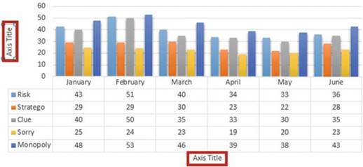
Figure13-21.Horizontalandverticalaxes
5.
Click the arrow for the Axis Title.
6.
We only want to use the horizontal Axis Title so select Primary Horizontal.
458
CHAPTER 13 ■ WORKING WITH CHARTS
Quick
Layouts
1.
On the Ribbon
under the Charts
Tools grouping, click the Design
tab. In the Chart Layouts
group click the Quick Layout button. See Figure 13-22.
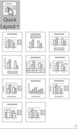
Figure 13-22. Options for Quick Layout
Excel has many predefined layouts that
contain different arrangements of your chart's elements.
2.
Move your cursor over each of the layouts to see how they
alter the look of your chart.
3.
Select Layout 3.
Changing
Chart Types
1.
In the Type group click the Change Chart Type button. A list of chart
categories appears in the left pane of the Change Chart Type window. The upper right pane contains
variations of the chart type selected in the left pane.
Clicking one of the variations displays the results
in the bottom right pane. See Figure 13-23. There are two available
charts in the lower right pane. The difference between
these is that one uses the column headings for the horizontal axis and the other chart uses the row headings
for the horizontal axis. Move your cursor over the two charts;
they will enlarge
so you can get a better view of them.
459
CHAPTER 13 ■ WORKING WITH CHARTS
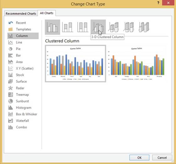
Figure 13-23.Charts available for the selected chart
appear in the bottom right pane
2.
Click Bar in the left pane. Click the first bar chart in the upper right pane which is a
clustered bar chart.
3.
Two clustered bar charts appear in the pane below. Click the chart on the right side.
4.
Click the OK button. See Figure 13-24.
460
CHAPTER 13 ■ WORKING WITH CHARTS
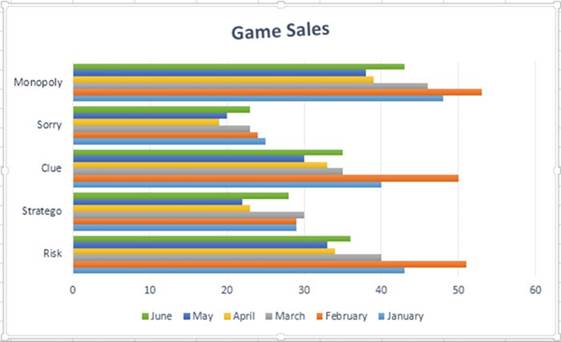
Figure13-24.ResultofselectingtheClusteredBarChart
Notice that the buttons in the Chart
Styles group and those in the Quick
Layout have changed
to reflect that the chart
is now a bar chart.
5.
In the Data Group, click the Switch Row/Column button.
The column headings
from the spreadsheet are now used for the vertical axis and the row headings
become the legend.
See Figure 13-25. This chart makes
it easier to see how much difference there was in sales for each individual game during the six-month
period.

Figure 13-25.The column headings
from the spreadsheet are the vertical
axis and the row headings
are the legend
461
CHAPTER 13 ■ WORKING WITH CHARTS
6.
Right-click the legend at the bottom of the chart and then select Format
Legend.
7.
Select Right from the Format Legend pane.
8.
In the Data Group on the Ribbon,
click the Select Data button.
This brings up the Select
Data Source dialog box shown in Figure 13-26.
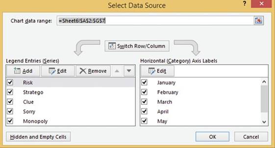
Figure13-26.SelectDataSourcedialogbox
The Select Data Source dialog
box provides you with an option for changing the range of cells that the chart
is based on. There is also a button here for switching the rows and columns just as you did in the previous
step.
There is an up and down arrow to the right
of the Remove button. These buttons as shown in Figure 13-27 are for moving
the current legend
up or down along with its
series.
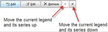
Figure13-27.Useupanddownbuttonstomovethecurrentlegend
Originally,
we had a column chart and the Risk game was represented by the first column in each month�s
group. When we changed to a bar chart, the series was reversed and the Risk game became
the last bar in each month�s group.
It seems strange
but in the Select Data Source dialog
box Risk is at the top even though it appears at the bottom
of a bar chart.
9.
With Risk selected, keep
clicking the down arrow shown in Figure 13-22 until
Risk becomes the last item in the
series.
462
CHAPTER 13 ■ WORKING WITH CHARTS
Risk now appears at the top of each month�s group in the bar chart.
10.
Click the check mark in front of Stratego to remove it.
11.
Click the check mark in front of June to remove it.
12.
Click the OK button.
Notice that no changes have been made to the spreadsheet data,
only to the chart. The legend and chart series
for Stratego have been removed
and all of the June data has been removed
from the chart.
13.
Let�s add another game to the spreadsheet. Add the line for the game Battleship as shown in Figure
13-28.
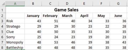
Figure13-28.Row8dataaddedtoworksheet
14.
Click the chart to select it. Click the Design tab on the Ribbon. In the Data group, click
the Select Data button.
15.
Click the Add button. The Edit Series dialog box appears.
16.
Click in the Series name text box.
17.
Click the word Battleship
in cell A8.
18.
Delete the text that is currently in the Series values: text box
19.
Drag across the cell range B8:G8 to get the sales data for
the Battleship game. See Figure 13-29.
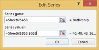
Figure13-29.DataenteredfortheEditSerieswindow
463
CHAPTER 13 ■ WORKING WITH CHARTS
20.
Click the OK button.
The chart should now show the monthly sales for Battleship.
21.
Click the OK button for the Select Data Source dialog box.
Changing a Series Color
The series color
for Risk and Monopoly are very close
and it is hard to distinguish one from another.
We will change the color
of the Risk series to red.
1.
On the Ribbon�s
Format tab, in the Current
Selection group, click the down arrow for Chart Elements
and then select Series �Risk.�
2.
In the Current Selection group, click
the Format Selection button.
3.
In the Format Data Series pane click the Fill & Line button
 . You can make a bar color a solid color, a gradient, or fill it with a pattern or a picture.
4.
Select Solid Color.
5.
Select the red color from the color picker button. See Figure 13-30.
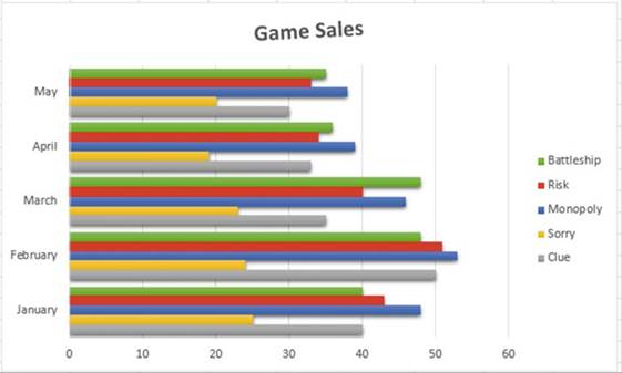
Figure 13-30.The
bars representing Risk have been changed to the color
red
You have learned how to create
column and bar charts. Column
and bar charts
work well for multiple columns
of numeric data.
Next you will learn how to create
pie charts. Pie charts should
only use a single column
of numeric data.
464
Pie Charts
CHAPTER 13 ■ WORKING WITH CHARTS
Pie charts are used to show percentages. The entire circle represents 100%. Each item in a data series is
represented by a slice of the pie. The size of each slice shows what part of the 100% it represents.
Sometimes you may find that the information in one slice needs to be broken out into percentages itself.
You can use the pie of pie subtype in such circumstances. In this section
we�ll first look at the standard pie chart and then cover the pie of pie subtype.
The
Standard Pie Chart
In Figure 13-31 we have ten pieces of fruit. The entire pie represents 100% of our fruit. There are five
bananas so they represent
5/10 or 50% of our fruit. Therefore, the bananas represent
one-half of our pie. The slice for Apples takes up 30% of the size of our pie.
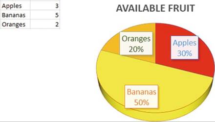
Figure 13-31. Pie chart with labels
In this exercise
you will create a pie chart from Dave�s Lunch Wagon data. A pie chart works well with this data because
there is only one column of label data and only one column of numeric data.
1.
Open workbook Chapter 13. Select the
worksheet named Pie.
2.
Select cells A2:B6. Click the Quick Analysis button at the bottom right of the data. See
Figure 13-32.
465
CHAPTER 13 ■ WORKING WITH CHARTS
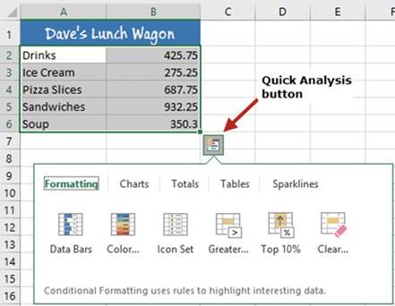
Figure13-32.OptionsforQuickAnalysisbutton
3.
Click Charts.
Excel recommends that you use a clustered
column chart, a pie chart, or a clustered bar chart for the data you have selected. If you were to click the
Clustered
Column button, Excel would create a clustered
column chart using the selected
data on the current worksheet.
4.
Move your cursor over the chart buttons to see how the
chart would look with your selected data.
5.
Click the pie chart. Click the chart.
6.
Click the Chart Styles button
 �to the right of the chart.
The Chart Styles box shows various
ways of displaying the current chart type. Let�s
select a chart that displays
the label and percent on each slice
of the pie. Having a label on each slice
of the pie makes having
a legend unnecessary.
7.
Click Pie Chart Style 10, which
you can see in Figure 13-33.
466
CHAPTER 13 ■ WORKING WITH CHARTS
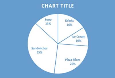
Figure13-33.PiechartwithPieChartStyle10applied
8.
Click CHART TITLE to select it.
9.
On the Ribbon�s Home tab, in the
Font group, change the font size to
28.
10.
Drag across CHART TITLE text to select it. Type Dave�s Chuck Wagon.
If the title appears on two lines,
then drag the bottom right
sizing handle of the chart frame (not the chart
title) to the bottom right
while you hold down the Shift key. Do this until Dave�s
Chuck Wagon displays
on only one line. See Figure 13-34.

Figure13-34.Titleshouldappearononeline
11.
Click Chart Title.
12.
Click the Chart Elements button
 �to the right of the
chart.
�to the right of the
chart.
13.
Move your cursor on Chart
Title. Click the arrow to the
right of it. Select More Options.
See Figure 13-35.
467
CHAPTER 13 ■ WORKING WITH CHARTS
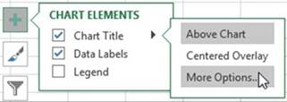
Figure13-35.SelectMoreOptionsfromtheChartTitleoptions
The
Format Chart Title
pane opens. There
are two options to choose from. The Title Options affects
the area inside the Chart Title area but outside the text itself. The Text Options affects only the
text.
14.
Click Text Options and complete the
following:
a.
Click the Text Effects button
 .
.
b.
Expand the Shadow option.
c.
Click the down arrow for Presets.
d.
Click the second shadow in the Outer group (Offset Bottom).
e.
Drag the Distance slider to 12 pt.
15.
Click the pie portion of the pie chart. The right pane should change to Format Data Series.
16.
Drag Angle of first slice slider to 26.
This will rotate the pie 26 degrees.
17.
To create some separation between
the pie slices,
change Pie Explosion to 2%. See Figure 13-36.
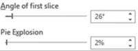
Figure 13-36.Change
Angle of first
slice to 26 and the Pie Explosion to 2%
The result should look like Figure 13-37.
468
CHAPTER 13 ■ WORKING WITH CHARTS

Figure13-37.Yourpiechartshouldnowlooklikethis
Pie of Pie Subtype
A pie of pie chart takes
a slice of a pie chart and then breaks
that slice into another pie chart. One reason for doing this is that your pie chart contains
too many items
and some of the pie slices are so small
that you
can�t tell what they are. Another reason
might be that one of the pie slices is a category
that you want further
broken down.
Annette owns a soup and sandwich
shop. She wants to see the breakdown
of her drink category. She wants to see what types of drinks customers
purchased this month. This can be done by pulling
the drink category
piece of the pie away from the others. This is called exploding the pie. You can explode
the entire pie or individual slices.
In this exercise
you will be creating a pie chart for a sandwich shop to show what percent
of sales are represented by sandwiches, soup,
ice cream, and drinks. The shop decided
that it would also like to see a break out of its drink sales to see what percentage of its drink sales is
represented by Pepsi, Coke, 7Up, and Sprite. You will create a pie of pie chart to display each of the
different types of drinks and then you will represent the same drink data with a bar of pie chart
1.
Open workbook Chapter 13. Click the worksheet tab Pie of Pie. Figure 13-38 shows
the worksheet data.
469
CHAPTER 13 ■ WORKING WITH CHARTS
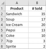
Figure13-38.DataontheworksheetPieofPie
When creating a pie of pie chart
Excel takes the items at the end of your selection for the second
pie chart so your data needs to be entered
accordingly.
2.
Select cell range A1:B8.
3.
On the Ribbon�s Insert tab, in
the Charts group, click the Pie Chart
button.
4.
Select the second
option (Pie of Pie) in the 2-D Pie area.
See Figure 13-39.
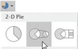
Figure 13-39. Select the Pie of Pie option
Excel took the last three
items by default
and made them the second
chart. See Figure
13-40. We are going to need to change that to the last four items.
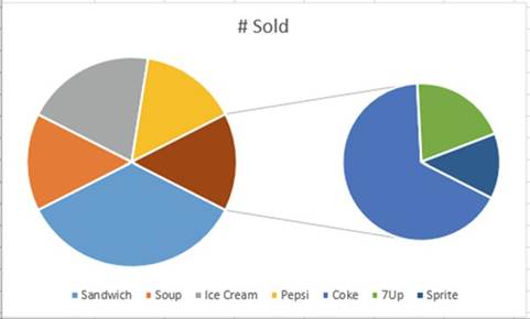
Figure13-40.Yourpiechartsshouldnowlooklikethis
470
CHAPTER 13 ■ WORKING WITH CHARTS
5.
Click the Chart. Click the Chart Element button.
6.
Move over Data Labels and then click the arrow to the right of it.
7.
Select Data Callout. See Figure 13-41.
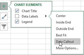
Figure13-41.SelectDataCalloutfromtheDataLabelsoptions
Figure 13-42 shows the result.
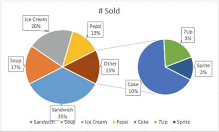
Figure13-42.Yourchartsshouldnowlooklikethis
8.
Double-click one of the pie slices from either chart.
This displays the Format Data Series pane on the right side of the spreadsheet.
9.
Click the Series Options button as shown in Figure 13-43.
471
CHAPTER 13 ■ WORKING WITH CHARTS
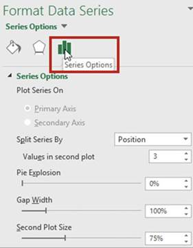
Figure 13-43. Select Series Options
The Split Series By combo box has four options. See Figure 13-44.
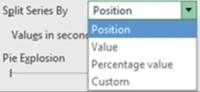
Figure 13-44. Options for Split Series By
The default value for Split Series
By is Position
and the default
Value for the combo box Values in second
plot is 3. These defaults
place the last three items
in the list on the second chart.
10.
Change the value
in Values in second
plot from 3 to 4. This moves
the Pepsi slice to the second chart.
See Figure 13-45.
472
CHAPTER 13 ■ WORKING WITH CHARTS
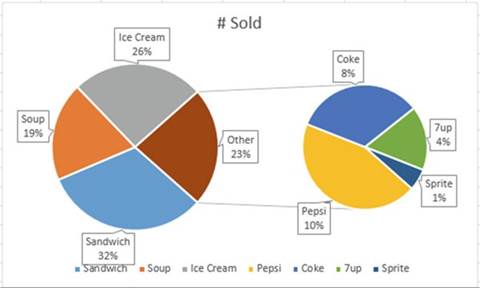
Figure13-45.ChangingtheValuesinsecondplotfrom3to4movedPepsitothepieofpiechart
You can use the other Split Series
By options to get the same results
as displayed in Figure 13-45. If you use the other
methods, you will not have to place
the items you want in the second
chart at the bottom of the list.
Changing
the value of Split Series By to Value
1.
Click the Undo button to undo moving Pepsi to the second chart.
For
this example, you
can get
the same
result by changing the Split Series
By to Value. When you select Value, Excel displays
a combo
box asking
for Values less than. Since Pepsi
has a
value of
13, you will
need to
change the value to 13.1
to move
the Pepsi
slice to
the second
chart.
2.
Select Value for the Split Series
By.
3.
Enter 13.1 for the Values less than.
See Figure 13-46.
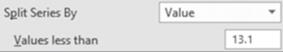
Figure 13-46.Select
Value for Split Series By and then Enter 13.1 for Values
less than
473
CHAPTER 13 ■ WORKING WITH CHARTS
Changing
the Value of Split Series By to Percentage Value
1.
Click the Undo button to undo moving Pepsi to the second chart.
Changing the option for the Split Series By combo box to Percentage
value brings up the Values less than combo box just as it
does when selecting Value. Pepsi on the chart displays a percentage
value of 13%. For this example, the values
and the percentages are the same because percentage values were used for the spreadsheet data. To move the
Pepsi slice to the second
chart we need to change the value in the Values
less than.
2.
Select Percentage value for the Split
Series By.
3.
Click on the up arrow for Values
less than until it is at 14. See
Figure 13-47.
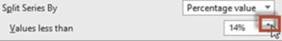
Figure
13-47.Select Percentage Value for Split Series By and then Enter 13.1 for Values
less than
Changing
the Value of Split Series By to Custom
1.
Click the Undo button to undo moving Pepsi to the second chart.
You can move slices from one chart to the other by selecting Custom from Split Series By and
then clicking the pie slice you want moved to the second chart and then selecting
which chart you want to move it to from the Point Belongs
to combo box.
2.
Select Custom value for the Split
Series By. See Figure 13-48.
474
CHAPTER 13 ■ WORKING WITH CHARTS
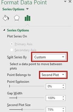
Figure 13-48. Select Custom for the Split Series By
3.
Double-click the Pepsi pie slice on the first chart. In the Point Belongs to drop-down box
select Second Plot.
4.
The chart shows that the four drinks
are part of the Other slice. The word Other doesn�t tell us anything. Select the word Other
and change
it to Drinks. See Figure 13-49. Click
inside a blank
area.
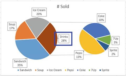
Figure 13-49. Changed the word Other to
Drinks
475
CHAPTER 13 ■ WORKING WITH CHARTS
5.
Click one of the charts.
Then in the Format Data Point pane, try
the following options:
�
The Pie Explosion is used for putting spacing
between the pie slices. The higher
the number the more the charts explode
out.
�
The Gap Width is used for changing the
amount of space between the two charts.
�
The Second Plot Size is used for changing the size of the second
chart.
Changing
Pie of Pie to Bar of Pie
The bar of
pie chart works the same way as the pie of pie chart.
1.
Select the Chart frame.
2.
On the Ribbon�s Insert tab, in
the Charts group, click the Pie Chart
button.
3.
Select the third option (Bar of Pie) in the 2-D Pie group. See Figure 13-50.
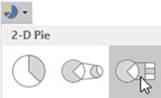
Figure13-50.SelectthethirdoptionBarofPie
Figure 13-51 shows the result.
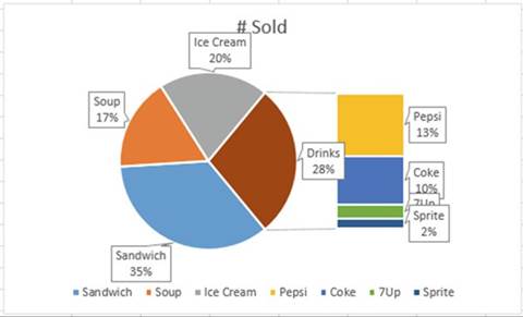
Figure13-51.Yourchartsshouldlooklikethis
476
CHAPTER 13 ■ WORKING WITH CHARTS
You have learned how to create
pie charts and even learned
how to break down a slice of the pie chart
into another pie chart or a bar chart. Next,
you will learn
how to combine two chart
types into a single chart called a Combination Chart.
Combination Chart
A combination chart combines more than one chart type in a single chart. The most common combination chart
consists of a bar chart for one series and a line chart for another
series. Figure 13-52 shows a combination where the sales data and predicted sales data are shown on the same
chart. The sales data is displayed
in a column format and the predicted
sales data in a line format. This makes it easy to see which predicted sales were higher and which predicted
sales were lower than the actual sales. Another reason for creating
a combination occurs when there is a large disparity
between the values in the different series.
Figure13-52.Combinationchartconsistingofacolumnandalinechart
In this example you will create a combination chart consisting of a column and a line chart.
Looking at Figure 13-53 you can see that there is a large disparity
in the values between the two columns.
As you will see this disparity prevents
us from creating an accurate
column chart.
1.
Open workbook Chapter
13. Select the worksheet named Combination. Figure
13-53 shows the data.
477
CHAPTER 13 ■ WORKING WITH CHARTS
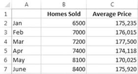
Figure13-53.DataintheworksheetnamedCombination
2.
Select the cell range A1:C7 and complete the following:
a.
Click the Quick Analysis button
at the bottom right of the selected data.
b.
Click the Charts tab.
c.
Click Clustered Column. Figure 13-54 shows the result.
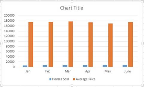
Figure 13-54. Clustered Column chart
You can see that this chart isn�t
very useful. There
is way too much disparity between the values
for Homes Sold and the Average Price.
3.
Click one of the Average Price columns in the chart to select the Average
Price series.
4.
On the Ribbon under Chart Tools click the Design
tab. In the Type group, click Change Chart Type.
5.
In the Change
Chart Type window select Combo in
the left
pane. Both series are displayed. The
Homes Sold
and the
Average Price are both
clustered columns.
6.
Click the down arrow for Clustered Column to the right of Average Price.
Under the Line group select Line with Markers. See Figure 13-55.
478
CHAPTER 13 ■ WORKING WITH CHARTS
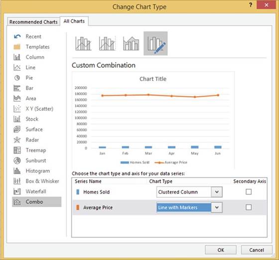
Figure 13-55. Select Line with Markers
7.
We need to create a second vertical
axis that will consist of values related
to the Average Price. The left vertical
axis will then show values
related to Homes
Sold.
a.
Check the Secondary Axis box to
the right of Average Price.
b.
Click the OK button.
8.
Click Chart Title.
Change the text to Number of Homes Sold and their Average Price. See Figure 13-56.
479
CHAPTER 13 ■ WORKING WITH CHARTS
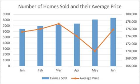
Figure 13-56. Chart with Title change
9.
So that the user can easily see that the values associated with the Average
Price are those on the right vertical
axis, let�s make them the same color as the line chart:
a.
Select Secondary Vertical
(Value) Axis.
b.
Click the Home tab.
c.
Click the Font Color�s down button.
d.
Select Orange, Accent 2, Darker 25%
e.
Click the Bold button. See Figure 13-57.
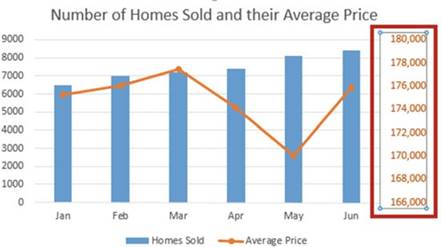
Figure13-57.TheverticalaxishasOrange,Accent2,Darker25%applied
You have learned how to combine
two chart types in a single combination chart. Next, you will learn how to create the two new hierarchical
charts for Excel 2016, the Treemap chart and the Sunburst chart.
480
Hierarchical
Charts
CHAPTER 13 ■ WORKING WITH CHARTS
Sometimes you will want to show the hierarchical relationships among
data. In this section, we�ll look at two common types of hierarchical charts:
the Treemap and Sunburst chart types.
Treemap Chart
A Treemap is used for representing hierarchical data. The chart
consists of rectangles whose size represents the value associated with a label.
Figure 13-59 shows a Treemap
chart.
In this exercise
you will create
a Treemap chart
using the data in Figure
13-58. Since the largest value
in the spreadsheet is 1000,
this item will be represented by the largest
rectangle. The rectangles representing the products
will be organized within the states.
1.
Open workbook Chapter 13. Select the
worksheet named Treemap.
Our company sells snack products to gas
stations in five states. Figure 13-58 shows our profit for the past week.
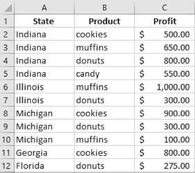
Figure13-58.DataintheworksheetnamedTreemap
A Treemap chart will give us a quick view of
the distribution of our profit for the various products across the five states.
■
NoteThe headings don�t
need to be selected when creating the chart.
2.
Select the range A2:C12. On the Ribbon�s
Insert tab click the See all Charts button in the bottom right corner of the Charts group.
3.
Select the All Charts tab and then select Treemap
in the left pane. Click the OK button. See Figure 13-59. The largest rectangle represents the largest
value.
481
CHAPTER 13 ■ WORKING WITH CHARTS
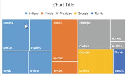
Figure 13-59. Treemap chart
It�s usually easier
to read a Treemap chart
if you turn the headings
(the state names
in this case)
to banners.
4.
Right-click any one of the rectangles on the chart
and then select
Format Data Series. Select
Banner from the Label
Options. See Figure
13-60.
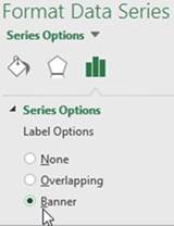
Figure13-60.SelectBannerfromtheLabelOptions
Figure 13-61 shows the result.
482
CHAPTER 13 ■ WORKING WITH CHARTS
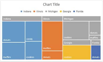
Figure13-61.Resultofchangingtheheadingstobanners
It�s easier to see the state headings
now. Since the Michigan Items are in gray, they blend in with the state headings
and are hard to read.
5.
Change colors of the rectangles:
a.
Click the Ribbon�s
Design tab. In the Chart
Styles group click
the Change Colors
button.
b.
Move your cursor over the different color
palettes to see how they affect your chart. We want one that doesn�t
have a gray color. Select
the third row in the Colorful group.
See Figure 13-62.
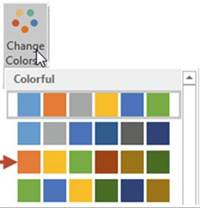
Figure13-62.SelectthethirdrowintheColorfulgroup
You might want to see the values along with the labels.
5.� Click the Chart
frame. Click the down arrow for Chart Options
and then select
Data Labels. See Figure 13-63.
483
CHAPTER 13 ■ WORKING WITH CHARTS
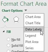
Figure13-63.SelectDataLabelsfromtheChartoptions
This adds another option button, Label
Options. See Figure 13-64.
Figure 13-64. Label Options
6.
Click the Label Options button.
Expand Label Options
so that you can see the options
as shown in Figure 13-65.
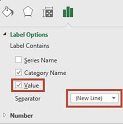
Figure 13-65. Label Options
7.
Select Value.
Select New Line from
the Separator drop-down box. Selecting New Line places
the label and the value
on two separate lines as shown in Figure 13-66.
484
CHAPTER 13 ■ WORKING WITH CHARTS
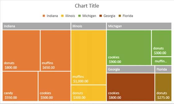
Figure 13-66.The labels and values should be on two separate
lines
8.
The white text can be hard to read:
a.
Click one of the labels
in the chart.
b.
Click the Ribbon�s
Format tab.
c.
In the WordArt Styles group click the down arrow
for Text Fill and then select the black color.
9.
With the labels still selected press Ctrl + B to bold the text.
10.
Click Chart Title. Drag across it to select it. Type Sales
by State.
If you triple-click a legend item or one of the rectangles, then all the rectangles not related to that item
will be dimmed. In Figure 13-67 the
legend item Michigan was triple-clicked. Once a group is selected you can
single-click an individual rectangle to
select it.
485
CHAPTER 13 ■ WORKING WITH CHARTS
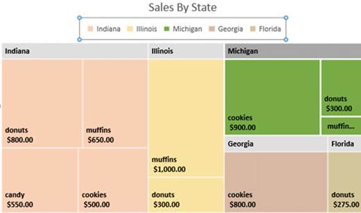
Figure 13-67.Michigan is highlighted because the
Michigan legend item was triple-clicked
11.
Triple-click the cookies
rectangle under Michigan
and then click donuts under Michigan. All rectangles should be dimmed except the Michigan donuts.
Click an empty cell to undim the rectangles.
When a group of rectangles or an individual rectangle is selected
you can change
its background to a different
color, gradient, picture,
or texture. Figure 13-68 shows that a texture was selected for the Michigan
group of rectangles. You can also apply various
effects and alter its borders
by clicking the Ribbon�s Format tab and then selecting one of the options from the Shapes
Styles group.
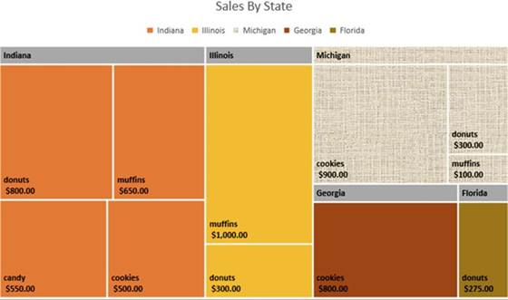
Figure13-68.TexturebackgroundwasselectedforMichigan
486
CHAPTER 13 ■ WORKING WITH CHARTS
12.
Triple-click the Michigan
cookies. In the Format Data Point pane on the right side click the Fill &
Line button (the paint bucket).
13.
Select Picture or texture fill.
14.
Click the drop-down box for Texture shown in Figure 13-69. Select whatever texture you want to
use.
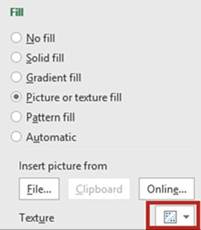
Figure 13-69. Select a texture
15.
Try changing the color or texture of
individual rectangles.
If not all of your data values are
showing you may need to expand the size of the chart.
Sunburst Chart
Like the Treemap chart the Sunburst chart is also a hierarchical chart. Instead of using the rectangle sizes
to represent a value, it uses the size of pie pieces.
An advantage of the Sunburst
chart over the Treemap chart is that it can represent more columns of labels. In the example
for the Treemap chart the first column
(State) was used for the headings and the next column (Product)
was used to represent the individual rectangles. If we wanted to break things down farther by going State,
then Counties,
and then Products
within those counties,
the Counties wouldn�t
display in the Treemap chart but they would in a Sunburst
chart.
Using the same data, we used for the Treemap
chart and selecting the same options,
let�s look at the result
for the Sunburst
chart in Figure
13-70.
487
CHAPTER 13 ■ WORKING WITH CHARTS
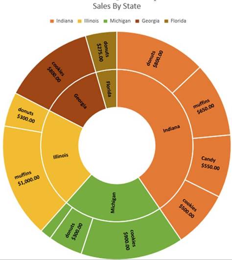
Figure 13-70. Sunburst chart
The Sunburst chart
clearly shows that Indiana is our most profitable state.
It�s easy to see from the chart that donuts are the most profitable item we sell in Indiana.
The pie slice
for muffins in Michigan isn�t
large enough to display the label and the value.
If we remove the values the label for the muffins
becomes visible. See Figure 13-71.
488
CHAPTER 13 ■ WORKING WITH CHARTS
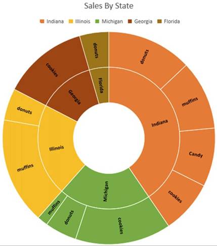
Figure 13-71.Removing the values gives more room for
the labels to display
The label for the muffins profit in Michigan
is now visible. See Figure
13-72. If you want to know the value
associated with each slice just move your cursor over one of the items.
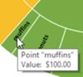
Figure 13-72.Move
your cursor over a slice
to see the associated value
489
CHAPTER 13 ■ WORKING WITH CHARTS
This exercise covers
selecting what data you wanted
represented in the Sunburst chart
as well as selecting portions
of the chart and applying
styles.
1.
Open workbook Chapter 13. Select the worksheet named Sunburst.
Figure 13-73 shows the data.
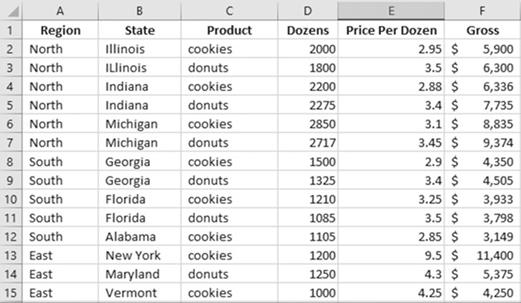
Figure13-73.DataintheworksheetnamedSunburst
2.
Select the cell range A2:D15 and complete the following:
a.
On the Ribbon�s
Insert tab, click
the dialog box launcher (See All Charts)
for the Charts group.
b.
Click the All Charts Tab.
c.
Select Sunburst in the left pane. Click
on the Ok button.
d.
Enlarge the chart. See Figure 13-74.
490
CHAPTER 13 ■ WORKING WITH CHARTS

Figure13-74.SunburstchartusingtherangeA2:D15
The Sunburst chart
makes it easy to see that we sell the most items
in the North region and that Indiana
and Michigan are the biggest
selling states.
What if we
wanted the chart to display the pie slices based on the Gross column?
3.
Delete the Sunburst chart.
4.
Select the cell range A2:C15,
hold down the Ctrl key and select the cell range F2:F15.
Let�s apply a cell style to the range so that we can easily identify which columns are being used for the
chart.
5.
On the Ribbon�s
Home tab in the Styles group, click
the Cell Styles button. Select
Accent5. See Figure
13-75.
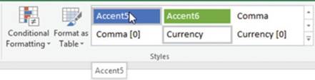
Figure13-75.SelectAccent5fromtheStylesgroup
491
CHAPTER 13 ■ WORKING WITH CHARTS
Your spreadsheet should look like Figure 13-76.
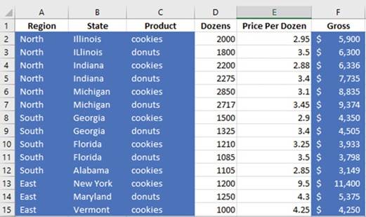
Figure13-76.Yourspreadsheetshouldnowlooklikethis.
6.
On the Ribbon�s
Insert tab, click
the dialog box launcher (See All Charts)
for the Charts group.
7.
Click the All Charts Tab. Select Sunburst
in the left pane. Click
on the OK button.
8.
Enlarge the chart. See Figure 13-77.
492
CHAPTER 13 ■ WORKING WITH CHARTS

Figure 13-77.Sunburst chart created from range A2:C15
and F2:F15 selected
We sell our product in New York City in a very upscale area at a higher price,
which makes our New York pie slice
much larger than it was for the number of dozens sold.
9.
Change the chart
to a more 3D-looking chart
by selecting the chart and then, from the Ribbon�s
Design tab, selecting the last chart
choice from the Chart Styles
group. See Figure
13-78.
493
CHAPTER 13 ■ WORKING WITH CHARTS

Figure13-78.Sunburstchartwith3Deffect
494
CHAPTER 13 ■ WORKING WITH CHARTS
Just like with the Treemap
chart you can select a group of pie slices
by triple-clicking one of the slices or a legend
item. You can then select
an individual slice
by clicking one of the slices in the selected
group. See Figure
13-79.

Figure13-79.SunburstchartwithNorthselected
You have learned how to create the Treemap
and Sunburst hierarchical charts. Hierarchical charts work
well for data where natural
groupings exist and the data is organized
in some level of order. Next, you will learn how to create charts that represent
a row of data and are stored in a single cell.
Sparklines
Sparklines
are small charts
displayed in individual cells. They are used for highlighting trends
within a� single row or single
column. There are three types
of sparklines: Line,
Column, and Win/Loss. Sparklines are created
by first selecting the cells where
you want the sparklines to be located
and then selecting the type of sparkline you want to create. The Sparklines group
is located on the Insert
tab. There are three buttons
in the group: Line, Column,
and Win/Loss. See Figure 13-80.
495
CHAPTER 13 ■ WORKING WITH CHARTS
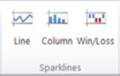
Figure13-80.Ribbon�sSparklinesgroup
Because the Sparklines are so small, if there isn�t a wide variance
in your values, the column charts may appear disproportionate in size compared
to the actual values. It is much easier to see the trends if you enlarge
the cell that contains the Sparklines.
Column sparklines that are negative
are displayed in the bottom half of the cell. Zero values are not given
a sparkline; instead,
a space is placed in that position.
See Figure 13-81.

Figure 13-81.Sparklines with negative values are displayed
at the bottom of the cell
Win/Loss sparklines show whether your data
is positive (win) or negative (loss). See Figure 13-82.
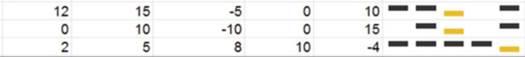
Figure13-82.Sparklinethatidentifieswinsandlosses
In this exercise
you will create sparklines for the row data in Figure 13-84. You will group and ungroup
the sparklines so that you can format some of your sparklines one way and some of them another
way
1.
Open the Chapter 13 workbook. Select the worksheet
named Sparklines. Figure 13-83 shows the data.
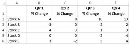
Figure13-83.DataintheworksheetnamedSparklines
496
CHAPTER 13 ■ WORKING WITH CHARTS
2.
On the Ribbon, on the Insert Tab, in
the Sparklines group, click the Line
button.
3.
Delete any text that is in the Data Range text box. Select the cell range B2:E6.
4.
Delete any text that is in the Location Range text box. Select the cell range F2:F6.
5.
Click the OK button.
6.
Under the Sparkline
Tools contextual tab, click the Design tab. In the Style group,
click the down arrow for more line color options.
Select the Sparkline
Style Colorful #4 in the last row. See Figure
13-84.
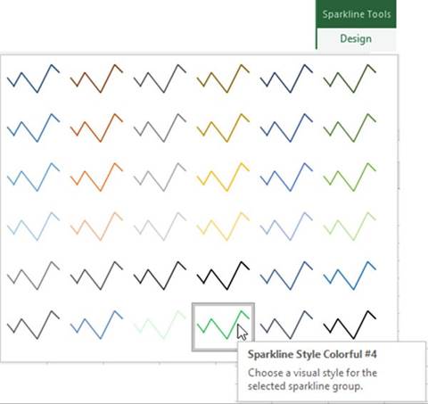
Figure13-84.SelectSparklineStyleColorful#4
7.
Drag across row heads 2, 3, 4, 5, and 6. On the Ribbon,
on the Home tab, in the Cells group, click
the Format button.
8.
Click Row Height. Change the
row height to 22. Click the OK
button.
9.
Change the column width for column F to 17.43.
10.
Select cells F2:F6.
11.
Under the Sparkline
Tools group, click the Design
tab. In the Show group click the High Point and Low Point check boxes. The Sparkline lines should now have
dots representing the highest and lowest points
on the line as shown in Figure
13-85.
497
CHAPTER 13 ■ WORKING WITH CHARTS
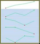
Figure13-85.Dotsrepresenthighestandlowestpoints
12.
Remove the check marks from the High Point and Low Point.
Check the Negative
Points. Now the points on the line represent those cells that have negative
values.
13.
Check the Markers. Now all the
cells are represented by points on the line.
14.
In the Style group, click
the Marker Color
button. Move your cursor over Markers. Select
purple from the Standard Colors.
See Figure 13-86.
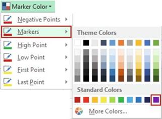
Figure13-86.SelectpurplefortheMarkercolor
15.
In the Style
group click the Marker Color
button. Move your cursor over Negative Points.
Select dark red from the Standard colors.
16.
In the Style group click the Sparkline
Color button. Move your cursor
over Weight. Select
the 4�-pt weight.
Changing the Weight
changes both the size of the line and the points. See Figure 13-87.
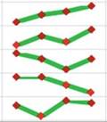
Figure13-87.Changingtheweightchangesthelineandpontsize
498
CHAPTER 13 ■ WORKING WITH CHARTS
17.
Click the Sparkline Color button again. In the
Theme colors select Blue, Accent
5, Lighter 40%
18.
In the Type group click Column. Let�s change the style. Click the More button for Style. Click
Sparkline Style Accent 5, Darker 25%. See Figure
13-88.
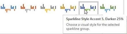
Figure 13-88. Select Sparkline Style Accent 5, Darker 25%
Ungrouping
Sparklines
1.
You may want some of your sparkline
cells formatted one way and some of the others
formatted another way. You can do this by grouping
and ungrouping the sparkline cells.
2.
Select cells F2 and F3.
3.
Click Ungroup. See Figure 13-89.
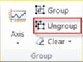
Figure 13-89. Click Ungroup
4.
In the Type group click
Line.
5.
In the Show group check off Markers and check on Last Point. See Figure 13-90.
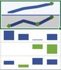
Figure 13-90. Last Point selected
499
CHAPTER 13 ■ WORKING WITH CHARTS
Grouping
Sparklines
1.
Select cells F2:F6. Click the Group button.
2.
Remove the check from Last Point.
3.
In the Type group click Win/Loss.
The points representing positive
values (wins) are displayed in the top half of the cell.
The points representing negative values (losses)
are displayed in the bottom
half of the cell.
Clearing
Sparklines
1.
Click cell F4.
2.
Click the down arrow to the right of the Clear button and
then click Clear Selected Sparklines. See Figure 13-91.
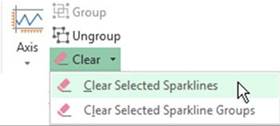
Figure 13-91. Select Clear Selected Sparklines
Changing
the Data Location and Location of the Sparklines
1.
Right-click column head B. Select Insert.
2.
Select cells G2:G6.
3.
Under Sparkline Tools click the
Design Tab.
4.
In the Sparkline group click the top half of the Edit Data button.
5.
Click the Collapse Dialog button to the right of the Data
Range text box. See Figure 13-92.
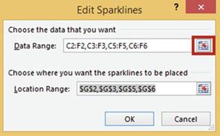
Figure13-92.ClicktheCollapseDialogbutton
500
CHAPTER 13 ■ WORKING WITH CHARTS
6.
Select Cells C2:F6. Click the
Expand Dialog button.
7.
Click the Collapse Dialog button to the right of the Location Range text
box.
8.
Select Cells B2:B6. Click the
Expand Dialog button.
9.
Click the OK button. See Figure 13-93.
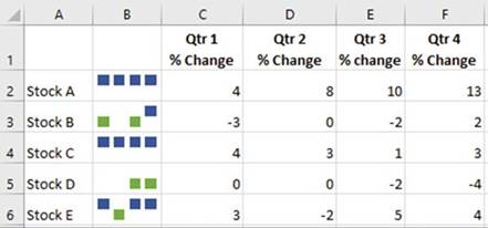
Figure13-93.Yourspreadsheetshouldnowlooklikethis
Summary
Charts provide a quick way of viewing
lots of data. They make it easy to see if you are meeting
your goals and to spot problems. What chart you use depends
upon the data that you want to represent. You have seen that column and bar charts can be used for many rows
of numeric data while a pie chart would represent
only one row of numeric
data. The Treemap
and Sunburst charts work well for representing hierarchal data. Sparklines are stored in an individual cell
and represent
a row of data. If you are using Sparklines, you will want to make the cell large enough so that you can
easily see what the chart is displaying.
Pie charts represent data in pie slices. The pie slices represent a percent of the entire pie. The Treemap
chart uses rectangles to represent values while a Sunburst chart represents values with pie pieces.
Sparklines can use one of three chart types: Line, Column,
or Win/Loss. A pie chart slice can be broken down into another pie or bar chart so that you can you see all
of the items that were used to create it.
A Combination chart combines
two charts into one. It usually consists
of a bar chart for one series and a line chart for another.
The fastest
way to create a 2D clustered bar chart is to use the following shortcut keys:
�
Press the Alt + F1 key if you want to display the chart on the same worksheet as the
data, or
�
Press F11 if you want the chart to appear on a separate
worksheet. The next chapter details
how to import data from various sources.
501
CHAPTER
14
Importing Data
Excel is the premier
analysis tool. This is the reason for bringing data from other sources into
Excel. Microsoft has added even more sources and ways of importing data for Excel
2016.
After
reading and working
through this chapter
you should be able to
�
Import delimited text and fixed-width text
files
�
Import data from an Access database
�
Import data as is from a web page and modify and transform it before importing it
�
Create connections between
a workbook and a data source
Importing Data
into Excel
Excel�s Ribbon has two
groups of buttons for bringing data into Excel. See Figure 14-1. The first group, Get External Data, is
strictly for
bringing data into a spreadsheet. The second group, Get & Transform, gives
you the opportunity to make
modifications to the data before bringing it in.
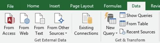
Figure14-1.GetExternalDatagroupandGet&Transformgroups
Excel can
import data from a wide variety of sources. The buttons in the Get External
Data group lets you
import data from text files, an Access database, the Web, XML files, SQL
server, and so on. It can even connect to other programs using an ODBC (Open Database Connectivity)
driver. The different file types do not all have the same capabilities in Excel. Some options work with some
data types and not with others.
503
CHAPTER 14 ■ IMPORTING DATA
Importing Text Files
Text files do not contain
any formatting. This makes it easy for different programs to exchange text file
data. There are two types of text files: delimited and fixed-width. The data in
a file is usually divided into fields. Delimited
files have fields that have variable lengths. All values in a fixed-width field
are the same length. Spaces are used to
make the length of text fields the same size; numeric fields can be padded with
zeroes to make them the same length.
Delimited Text Files
Fields in text files are usually
separated by commas but they can also be separated by tabs, spaces, or any other character. The character
used to
separate the fields is called the delimiter. A text file that has its fields separated by commas is called a
comma-delimited text file. Most text files have an extension of .txt. Excel spreadsheets can be saved as
text
files with an extension of .csv. The extension stands for comma separated values.
Following is the content
from a comma-delimited file. The file has headings in the first
row. Not all text files contain a header row.
EmployeeID,DeptID,LastName,FirstName,MidInitial
A3251,05,Carson,Annette,F A3291,04,Sterk,Carrie,M A1450,04,Uhrhammer,Dorothy,L
A1425,05,Carson,Dick,J
In this exercise
you will import
data from a delimited text file into a worksheet. You will create
two connections to the text file. One connection will automatically refresh
the worksheet with any updated
data from the text file when the file is open and the other
connection will not. You will also learn
to import just the data that you want to be imported.
1.
Create a new blank workbook named �ImportingData.�
2.
Click the Ribbon�s
Data tab. In the Get External Data group click
From Text.
3.
This brings up the Import
Text File window where you browse until you find the file. Select the Employee.txt file and then select the
Import button.
4.
This brings up the Text Import
Wizard � Step 1 of 3 window. See Figure 14-2. Since this file is a comma-delimited file you need to
make sure Delimited is selected. The file has headers so select My Data has headers.
504
CHAPTER 14 ■ IMPORTING DATA
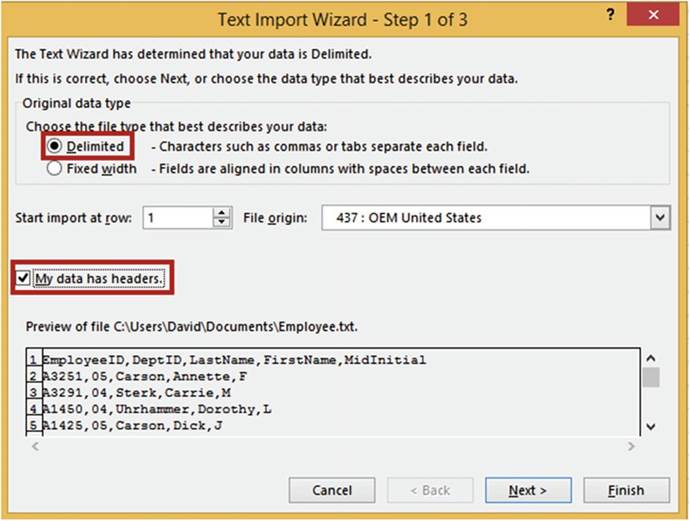
Figure14-2.TextImportWizard-Step1of3
5.
Click the Next button.
The Text Import Wizard � Step 2 of 3 window
opens. See Figure 14-3.
6.
Under Delimiters deselect Tab
and select Comma.
Notice that when you select Comma, the data in the Data preview area automatically separates into columns.
505
CHAPTER 14 ■ IMPORTING DATA
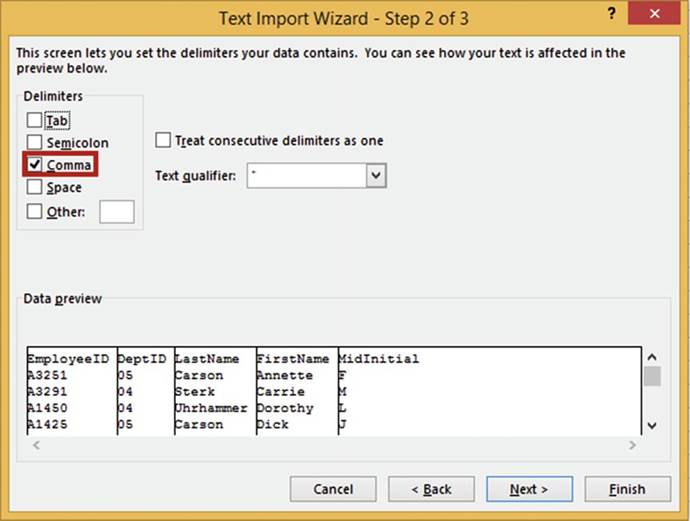
Figure14-3.TextImpoortWizard�Step2of3
7.
Click the Next button.
The Text Import Wizard
� Step 3 of 3 window opens.
See Figure 14-4. This window has options for selecting the data format
for each field
as well as for preventing fields you select
from being imported
into your worksheet. We don�t want to import
the DeptID field
and the MidInitial fields.
8.
Click anywhere within the DeptID column and then select Do not import column (skip).
9.
Click anywhere within the MidInitial column and then select
Do not import column (skip).
The headings above the fields you selected
not to import changed from General to Skip Column.
506
CHAPTER 14 ■ IMPORTING DATA
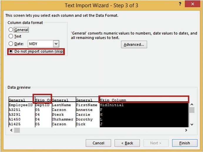
Figure14-4.TextImportWizard�Step3of3
10.
Click the Finish button.
The Import Data window opens. See Figure
14-5. Text files can only be shown in Table view. You can specify
the beginning cell location in this window
and change various
properties.
507
CHAPTER 14 ■ IMPORTING DATA
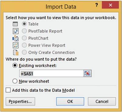
Figure 14-5. Import Data dialog
box
11.
Leave the location as cell A1. Click the Properties button.
Creating a
Connection to the External Data
The External Data Range Properties dialog box opens.
See Figure 14-6. One of the changes you can make in this window is how often or when the file is updated.
For example, you could set the Refresh
control to refresh
every ten minutes.
You could then make a change to the data in the Employee. txt file, wait ten minutes, and then see the
changes
displayed in the worksheet, or you could set it to refresh
when you reopen the workbook.
508
CHAPTER 14 ■ IMPORTING DATA
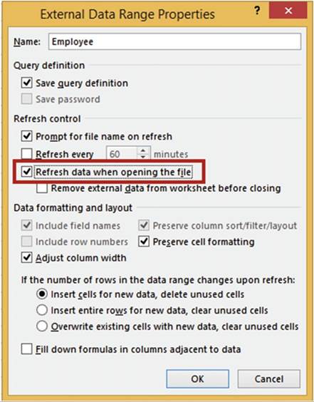
Figure14-6.ExternalDataRangePropertiesdialogbox
1.
Select Refresh data when opening
the file. Click the OK button.
2.
Click the OK button on the Import Data dialog box.
The imported data is now a part of the
worksheet and a connection has been created
to the data. See Figure 14-7.
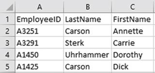
Figure14-7.Importeddataisnowpartoftheworksheet
509
CHAPTER 14 ■ IMPORTING DATA
3.
Click a blank cell.
4.
On the Ribbon select the Data tab; in the Get External
Data group click Existing Connections.
The Existing Connections window opens. See Figure 14-8. This window shows any connections you have in the
current
workbook, on your network, and on your computer. Currently we just have a connection to the Employee
text file in our workbook.
Now that we have a connection we can keep using this data without
having to create
another connection.
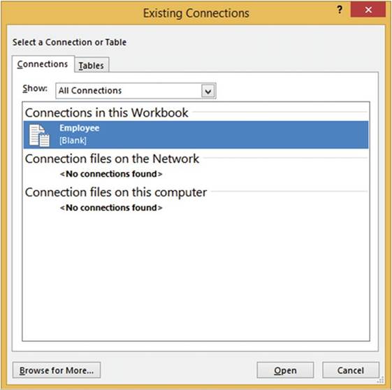
Figure14-8.ExistingConnectionsdialogbox
510
CHAPTER 14 ■ IMPORTING DATA
Creating a
Second Connection to the Employee.txt File
1.
Click cell D7. If the Existing
Connections window is covering cell D7, move
it.
2.
Double-click the Employee file or click the Open button.
The Import Data window opens.
See Figure 14-9. You can place the data in another
location or another
worksheet.
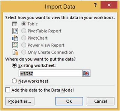
Figure14-9.Specifywhereyouwanttheimporteddataplaced
3.
Leave the Existing
worksheet cell at D7.
This time we won�t click the Properties
button where we set the first connection to refresh the data when opening the
file.
4.
Click the OK button.
Another copy
of the file from the first connection displays starting in cell D7.
5.
Click a blank cell.
6.
On the Ribbon select the Data tab; in the Get External
Data group click Existing Connections.
The Existing Connections
dialog box opens. Excel
named the second connection Employee1. See Figure 14-10.
511
CHAPTER 14 ■ IMPORTING DATA
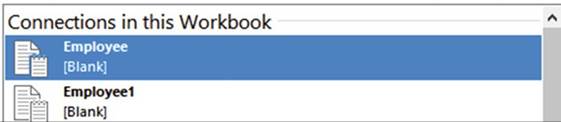
Figure14-10.Connectionstoimportedfiles
7.
Click the Cancel button.
Because the second connection�s property isn�t set to
refresh when the file is opened, any
changes made to the Employee.txt file will not affect
the second connections copy of the
data on the worksheet when the workbook is opened.
8.
Save this workbook. Close the workbook.
9.
Use Notepad or WordPad to change the Employee.txt file so that the first EmployeeID is A9999
rather than A3251. Save the Employee.txt file.
10.
Reopen the ImportingData workbook.
You may get a security
warning above your worksheet. If you do, click the Enable Content
button.
11.
The Import Text File
dialog box opens. See
Figure 14-11. It opens because we
left the
Prompt
for file
name on
refresh selected in the External
Data Range
Properties window. With Employee selected
for the
File name
click the
Import button.
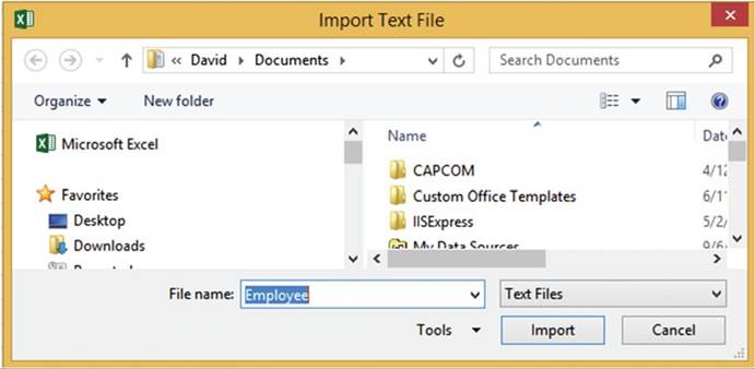
Figure 14-11. Import Text File dialog box
512
CHAPTER 14 ■ IMPORTING DATA
Figure 14-12 shows that the EmployeeID in cell A2 has been changed to the same value you updated it to in the
Employee.txt file. The value
in cell D8 kept the original value.
The reason this occurred was because in the first
connection we selected
the property for Refresh
data when opening
the file.
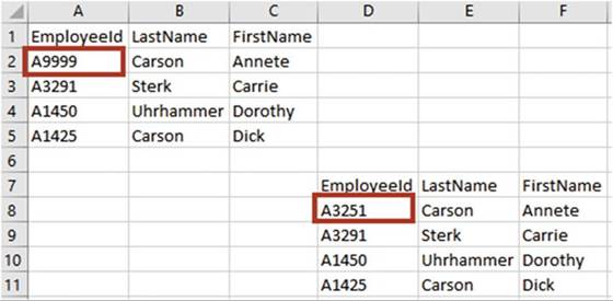
Figure 14-12.EmployeeId in cell A2 was changed
to the value you updated
it to in the Employee.txt file
12.
If you want to refresh the data for all the connections
immediately, click the Refresh All button. See Figure 14-13.
Figure 14-13. Refresh All button
13.
On the Ribbon
select the Data tab; in the Connections group click the Refresh All button. The Import Text dialog box
appears again.
14.
With Employee entered for the File name click the Import
button. Since there are two connections you will have to do this
twice.
The data
from both connections should now match.
513
CHAPTER 14 ■ IMPORTING DATA
Breaking the
Connection Between �the Imported File and Your Workbook
What if you didn�t want Excel to update the data any more when a change
was made to the file?
1.
On the Ribbon�s Data tab; in the
Connections group,
click
the Connections button. The Workbook Connections dialog box opens. See Figure 14-14.
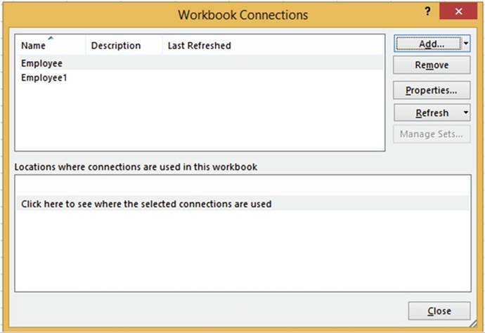
Figure14-14.WorkbookConnectionsdialogbox
From this dialog box you can Add and Remove connections and change their
properties. The bottom
half of the dialog box has an option to find where
the connections are used.
2.
Remove the first data connection by selecting Employee and
then clicking the Remove button.
3.
You will get a warning
that you will separate the workbook from its data source. Click the OK button. The Employee connection is
removed.
4.
Click the Close button.
5.
Change the Employee.txt file so that
the first Employee ID is A0000. Save the file.
514
CHAPTER 14 ■ IMPORTING DATA
6.
On the Ribbon�s Data tab, in
the Connections group, click the
Refresh All button.
7.
The Import Text dialog box appears again.
With Employee entered
for the File name click
the Import button.
Because the first
connection was removed
there was no change to the EmployeeID, but the other
data set was updated. See Figure 14-15.
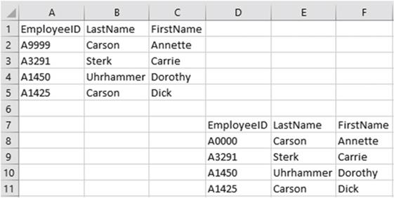
Figure 14-15. Updated data
Changing What
Data Is Being Imported
1.
On the Ribbon,
in the Data tab, in the Connections group click the Connections button.
2.
Click the Properties button. The
Connection Properties window
displays. See Figure
14-16.
3.
Employee1 isn�t a very good name; change it to Employee_Updated.
4.
For the Description, enter Uses the Employee.txt file. Updated with Refresh All.
Notice that Refresh this connection on Refresh All is selected.
515
CHAPTER 14 ■ IMPORTING DATA
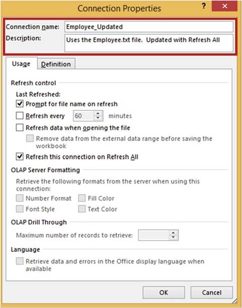
Figure14-16.ConnectionPropertiesdialogbox
5.
Click the Definition tab. Click the Edit Query button.
6.
Make sure that Employee is selected for the File name in the Import
Text File dialog
box.
7.
Click the Import button.
8.
For Step 1 of the Text Import Wizard click the Next button.
9.
For Step 2 of the Text Import Wizard click the Next button.
10.
For Step 3 of the Text Import
Wizard click anywhere
in the EmployeeID column and then select Do not import column (skip).
11.
Click anywhere in the DeptID column and then select General. See Figure 14-17.
516
CHAPTER 14 ■ IMPORTING DATA
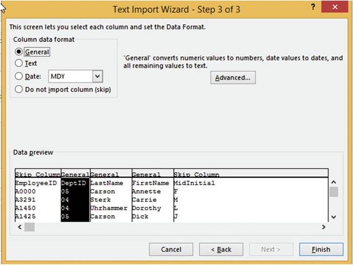
Figure14-17.TextImportWizard�Step3of3
12.
Click the Finish button.
13.
Click OK on the Connection Properties window.
14.
Click Close on the Workbook
Connections dialog box.
517
CHAPTER 14 ■ IMPORTING DATA
The edited query changes the connected data. See Figure 14-18.
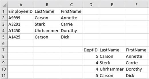
Figure14-18.Connecteddatahaschanged
15.
Click the Close button on the Workbook
Connections dialog box.
You have learned how to import delimited files. The fields can be delimited by commas, semicolons,
and so on. There doesn�t need to be spaces between fields in a delimited file. Next you will learn how to
import fixed-width text files. In a fixed-width text file, there is no delimiter. The fields are separated
by spaces.
Fixed-Width Text Files
In a fixed-width text file all fields take up the same amount of space. Headings aren�t usually used because
they would rarely line up with the data.
A3251 05 Carson��� Annette F
A3291
04 Sterk��� Carrie M A1450 04 Uhrhammer�� Dorothy L A1425 05 Carson��� Dick� J
Importing a fixed-width text file is almost identical
to importing a delimited text file.
518
CHAPTER 14 ■ IMPORTING DATA
In this exercise you will import data from a
text file stored in fixed-width format into a location that you specify in your
worksheet.
1.
Create a new worksheet named �Fixed-Width.�
2.
On the Ribbon select the Data tab; in the Get External
Data group click From Text.
3.
This brings up the Import Text File dialog box where you
browse until you find the file. Select the file Employee_Fixed.txt and then select the Import button.
4.
This brings up the Text Import Wizard.
See Figure 14-19. Excel recognized this as a fixed-width file and automatically selected that option.
5.
Click the Next button.
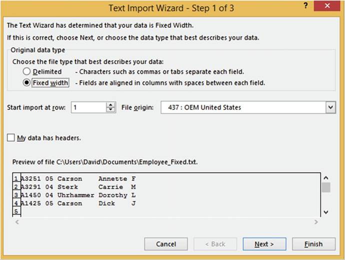
Figure14-19.TextImportWizard�Step1of3
519
CHAPTER 14 ■ IMPORTING DATA
6.
Click the Next button. This
brings up the second step. See
Figure 14-20.
The fields in a fixed-width file can be separated wherever
you want them to be, by dragging
the lines. You could combine
fields by double-clicking the line between
them to remove
it. You could
create another column
between columns by clicking where
you want to create the extra lines.
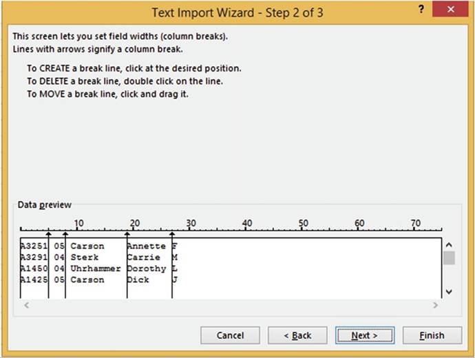
Figure14-20.TextImportWizard�Step2of3
7.
Click the Next button for Step 2.
8.
Click the Finish button for Step 3
The Import Data dialog box displays. See Figure 14-21. Here you can specify the location of where you want
the data loaded in the current workbook
or if you want it placed in a new worksheet.
9.
Select cell A3. Click the OK button.
520
CHAPTER 14 ■ IMPORTING DATA
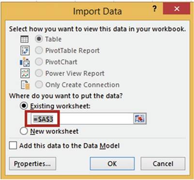
Figure 14-21. Import Data window
The data is
imported starting in cell A3. See Figure 14-22.
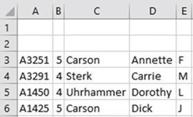
Figure 14-22. Imported data
You have learned how to import
text files. Next you will learn how to import
data from an Access database.
Importing Data
from an Access Database
Microsoft Access is a part
of the Microsoft Office suite. An Access database can contain multiple linked tables and queries. A query
contains
only the fields from a table that you requested. The records it contains are limited to any filters you
placed
on it. You can import data from tables and queries that you have created in Access.
521
CHAPTER 14 ■ IMPORTING DATA
In this exercise
you will import
the data from a table
named tblCustomer, which
is in the Access database
named Customers.
1.
Create a new worksheet named
�Access.�
2.
Click the Ribbon�s Data tab. In the Get External
Data group, click
the From Access
button. The Select Data Source dialog box opens.
3.
Select the Access
database named Customers and then click
the Open button.
See Figure 14-23.
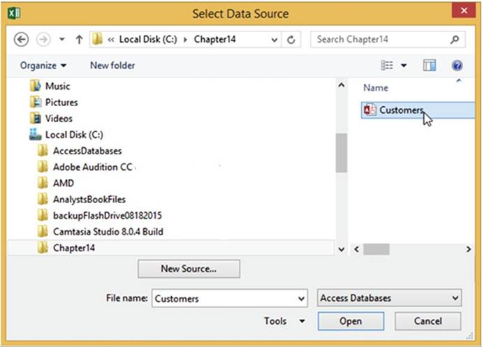
Figure 14-23.Select the Access database to be opened
4.
The
Customers Access Database contains two tables:
tblCustomer and tblOrderinfo. It also contains a query named qryCustomerbyState.
See Figure 14-24. Select the table named tblCustomer
from the Select
Table
dialog box. If you wanted to import more than one table or query you would need to check the Enable
selection of multiple tables.
5.
Click the OK button.
522
CHAPTER 14 ■ IMPORTING DATA
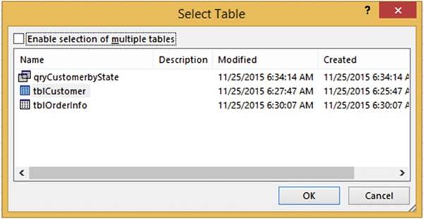
Figure14-24.Selectthetableorqueryyouwanttoimport
6.
In the Import Data dialog
box you need to specify
how you want to view the data and where
you want to locate it in your workbook. With the cursor
in the Existing worksheet text box click
cell A2. See Figure 14-25. Click
the OK button.
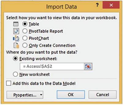
Figure14-25.Selecthowyouwanttoviewthedataandwheretoputit
The data you selected is placed in a table in your workbook. See Figure 14-26. If you want to update the
imported
data in your Excel workbook
after you have made a change to the data in Access,
then right- click anywhere in the table and select Refresh.
523
CHAPTER 14 ■ IMPORTING DATA
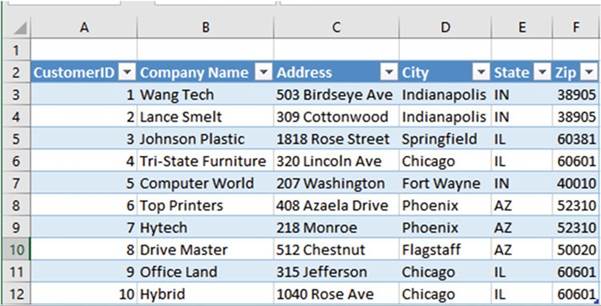
Figure14-26.Datahasbeenimportedintoatable
Importing Data from a Web Site
A web site is
another source from which you can import data into Excel. In this section you
will import tables from a
web page exactly as they appear in the web page. As with other data sources,
you also can use a query, which is covered in the next section.

In this exercise you will import two tables from a web site into a
worksheet.
1.
Add a new worksheet to the Importing Data workbook you
created in the first practice for this chapter.
2.
Click the Ribbon�s Data tab. In the Get External
Data group, click the From Web
button. The New
Web Query dialog box opens. See
Figure 14-27.
3.
In the Address box, enter http://professoroffice.com/tables.htm.
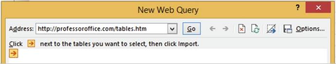
Figure14-27.NewWebQuerydialogbox
524
CHAPTER 14 ■ IMPORTING DATA
Notice that the instructions say that you
should click the
 �next to the table you want to select.
4.
Press Enter or click the Go button
The New Web Query dialog
box now contains the web site you entered. There
are two tables on this web page. There is an arrow to the left of each table and one arrow at the top.
Clicking the top arrow selects both tables. Clicking
the arrow to the left of a table selects
just that table.
5.
Click the top arrow as shown in Figure 14-28. The
arrow turns into a check mark
 .
.
6.
Click the Import button at the bottom of the dialog box.
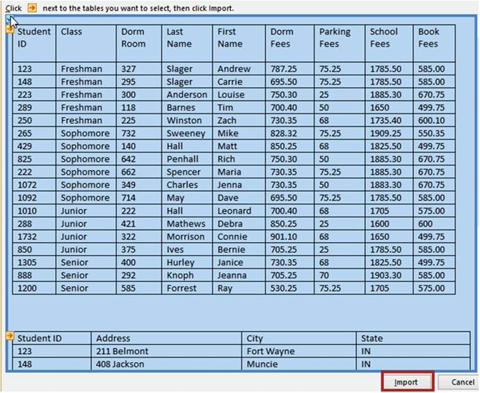
Figure14-28.Bothtablesareselected
525
CHAPTER 14 ■ IMPORTING DATA
Excel asks you where you want to import the data. See Figure 14-29.
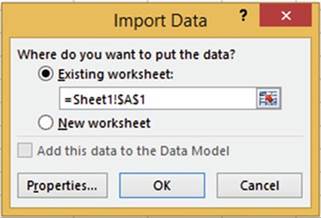
Figure14-29.Selectwhereyouwanttostoretheimporteddata
7.
Leave the location as cell A1 in
the current worksheet. Click the OK
button.
The data
has now been imported into your spreadsheet and you can manipulate it any way
you wish. See Figure 14-30.
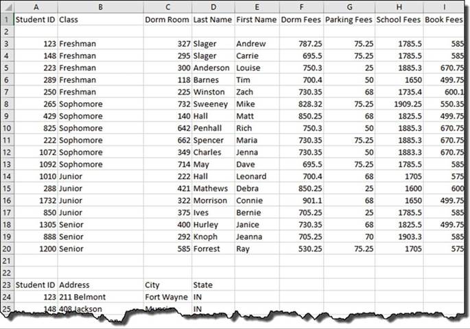
Figure
14-30. Imported data

526
CHAPTER 14 ■ IMPORTING DATA
You have
learned how you can import data directly into Excel from tables you find on the
Internet. Next, you will learn how to use Excel�s new Queryfeature. This feature lets you select only
the fields and
data that you want to import. You can
even add your own calculated fields.
Importing Data Using
a Query
Excel�s new Queryfeature can bring in data from many sources and it has the
ability to do a great deal of modification to your data. Among the sources from which you can import data
are web pages and
databases. Excel enables you to import data from a variety of
database types by default. You can use any data source that is
available from the New Query button on the Ribbon�s Data tab.
■
Note� You also
can import
data from
other sources,
such as various database management systems
(DBMSs) via the ODBC standard. You can get ODBC and
other data
source drivers from third parties.
In
this section, you will import
data from a web page using a query from the Get & Transform group.
In this
exercise you will choose which fields you want to import. You will filter the data, create a
calculated column, merge the
queried data and change the order of the columns.
1.
Add a new worksheet to the Importing Data workbook you created in Exercise
14-1.
2.
Click the Ribbon�s
Data tab. In the
Get & Transform group, click the New Query
button.
3.
Click From Other Sources
and then select
From Web. The New Web Query window opens.
4.
In the URL (uniform resource locator) text box enter http://professoroffice. com/tables.htm. See
Figure 14-31.
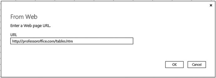
Figure14-31.EnterthewebaddressintheURLtextbox
527
CHAPTER 14 ■ IMPORTING DATA
5.
Click the OK button.
The Navigator window displays. See Figure 14-32. The two tables
from the web page are now available. Excel named the tables Table0
and Table1. Clicking
a table name in the left pane displays that table in the right pane. If you want to select
more than one table, you need to check Select multiple
items.
At the bottom of the window there is a Load
and Edit button. If you want to
import the data into your worksheet just the way it is you could click the Load
button.
Clicking the Edit button gives you the
opportunity to modify the data and limit what data is brought in before it is
imported into your worksheet.
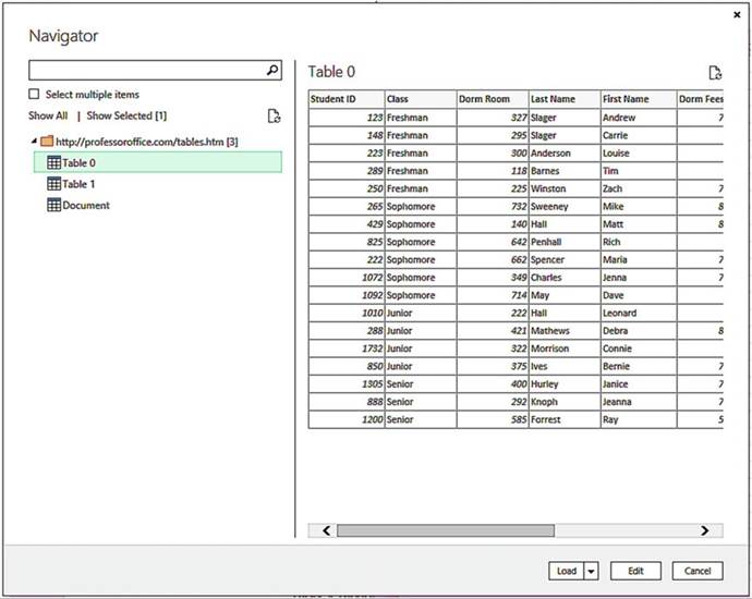
Figure 14-32.Selecting a table from the left pane displays
it in the right pane
528
CHAPTER 14 ■ IMPORTING DATA
6.
Check Select multiple items. Check Table0 and Table1. See Figure 14-33.
7.
Click the Edit button.
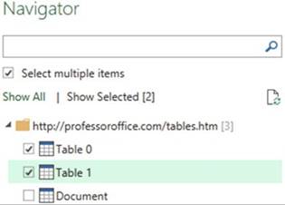
Figure14-33.SelectmultipleitemsandTable0andTable1
Naming the Tables
1.
The Query Editor
displays. The
Query Settings
pane is
on the
right side
of the
screen. Change the table name from
Table0 to tblStudentFees. Press Enter. See Figure 14-34.
Figure14-34.ChangethenametotblStudentFees
2.
Click Table1 on the left side of the screen.
Change its name in the Query Settings
pane to tblStudentAddress. Press Enter.
Choose
Fields to Import
We don�t
need the Address column in the
tblStudentAddress table.
3.
Click the Address column head to select the entire column.
In the Ribbon�s Manage Columns group there is a Remove
Columns button. Clicking the top half of the button removes the currently selected column.
Clicking the bottom half of the button provides two options.
One option is Remove Columns, which does the same thing as clicking the top half of the button. Clicking the
second option,
Remove
Other Columns, removes all of the columns except the currently selected ones.
529
CHAPTER 14 ■ IMPORTING DATA
4.
Click the top half of the Remove Columns button.
5.
On the left side of the window, click table tblStudentFees.
We don�t need the column Dorm
Room from this table.
6.
Click the Dorm Room column
head.
7.
In the Ribbon�s
Manage Columns group,
click the top half of the Remove Columns button.
Applying
a Filter
We only want
to import records of students whose parking fees are greater than $25.
1.
Click the down arrow to the right of the Parking Fees column heading.
2.
Click Number Filters.
Select Greater Than.
The Filter Rows window
appears.
3.
Click the down arrow for the second drop-down box. This drop-down box displays all of the values
in the column. See Figure 14-35.
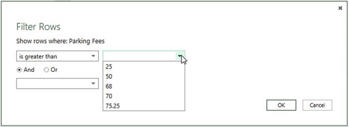
Figure14-35.Select25afterselectingisgreterthan
4.
Select 25. Click the OK button. All records with 25 or less for the parking
fees are removed.
Three records were removed.
5.
On the left side of the window click the tblStudentAddress table.
6.
Click the down arrow to the right of the State column heading.
7.
Uncheck IL. Click
the OK button. The four records that contained the state of IL are removed.
530
CHAPTER 14 ■ IMPORTING DATA
Undoing and
Redoing Query Steps
The Applied Steps area in the Query Settings pane keeps track of all the changes
you make to the query.
If you want to see what your query looked
like before your last step you can click the step above it. As you move up in the Applied
Steps you are basically performing an Undo. Click
the line below the current
one if you want to Redo the step.
1.
In the APPLIED STEPS area, click Removed Columns. See Figure 14-36
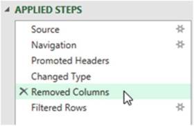
Figure14-36.SelectRemovedColumns
The records that contained the state of IL are displayed again.
2.
In the left pane click the tblStudentFees table. In the
APPLIED STEPS area, click Removed Columns.
The records
that contained parking fees of 25 or less are displayed again.
3.
Click Filtered Rows. The filter
is reapplied and those records
that contained parking
fees of 25 or less are no longer displayed.
�
Right-clicking an applied step brings up the menu options
shown in Figure 14-37. From here you can elect to do the
following:
�
Edit the settings
you created. For example, this step could
be edited from only showing
records where the parking fee is greater
than 25 to greater than 50 or whatever you want.
�
Rename a step.
�
Delete a step. If you delete it, you
can�t get the step back.
�
Delete all the steps from the current
step to the last step.
�
Move steps up and down to change their
order.
531
CHAPTER 14 ■ IMPORTING DATA
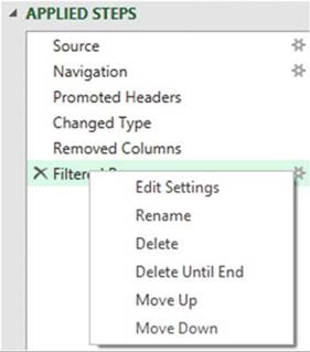
Figure14-37.Right-clickasteptoviewitsoptions
Creating
a Calculated Column
1.
Click the Ribbon�s
Add Column tab. In the General group, click the Add Custom Column
button.
2.
You may get the message in Figure 14-38. If
you do click the Insert button.
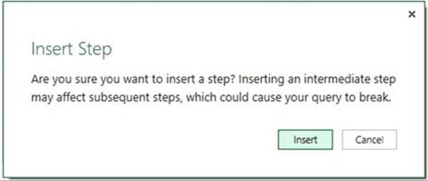
Figure14-38.InsertStepmessage
532
CHAPTER 14 ■ IMPORTING DATA
3.
Enter TotalFees for the New Column name in the Add Custom
Column dialog box and complete
the following steps. See Figure 14-39.
a.
In the Available columns list box, double-click Dorm Fees.
b.
Enter a plus sign (+).
c.
Double-click Parking Fees.
d.
Enter a plus sign (+).
e.
Double-click School Fees.
f.
Enter a plus sign (+).
g.
Double-click Book Fees.
h.
Click the OK button.
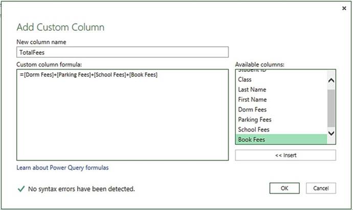
Figure 14-39. Add a custom
column
533
CHAPTER 14 ■ IMPORTING DATA
4.
Click the down arrow to the right of the
Total Fees field. Select Sort
Descending.
The reason Excel creates the applied steps
is so that the next time you want to do an import from the web page, you will not have go through this
editing process
again. The steps
will be saved
and automatically run for you.
Merging
Queries
1.
Click the Ribbon�s Home tab. In
the Combine group, click the Merge
Queries button.
The Merge window
displays with the data from tblStudentFees displaying at the top.
2.
Select tblStudentAddress from the drop-down box as shown in
Figure 14-40. We will link the tables together and then
we will add the fields we want from the tblStudentAddress
field.
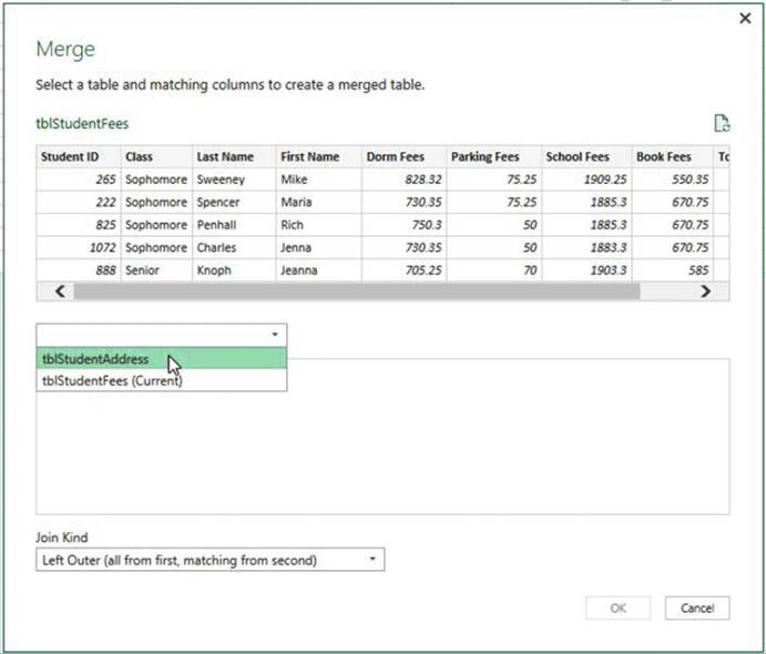
Figure14-40.SelecttblStudentAddress
534
CHAPTER 14 ■ IMPORTING DATA
3.
Click the Student
ID column head in both tables. See Figure 14-41. This links the two tables.
Both tables have the same Student ID numbers.
4.
Click inside the check box for Only
include matching rows.
Twelve of the records in tblStudentFees have a matching
record in tblStudentAddress. Because you selected
Inner(only matching rows) only the records with matching Student
IDs will become
part of the query.
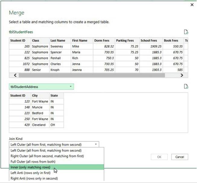
Figure14-41.ClicktheStudentIDcolumnheadinbothtablestolinkthetwotables
535
CHAPTER 14 ■ IMPORTING DATA
5.
Click the OK button.
A new column appears at the end of the tblStudentFees table.
Each row in the column contains the word Table. See Figure 14-42.
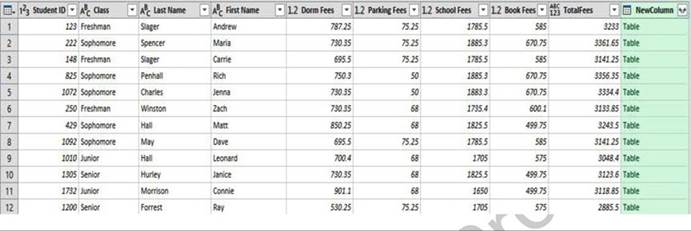
Figure14-42.Anewcolumnisdisplayedtotherightofthetable
To the right of the
NewColumn header there is a column expansion button. See Figure 14-43. We want to add the City and State
fields from the tblStudentAddress table but not the StudentID. The merged table already
contains a StudentID so that
would
be redundant.
6.
Click the Column Expansion button. Uncheck
Student ID.
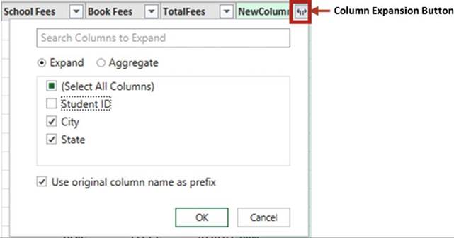
Figure14-43.ClicktheColumnExpansionbuttonanduncheckStudentID
536
CHAPTER 14 ■ IMPORTING DATA
7.
Click the OK button.
The City and State columns
have been added
to the table. We would like to remove the word NewColumn from
the City and State columns.
See Figure 14-44.
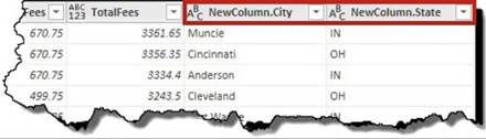
Figure 14-44.Remove the word NewColumn from the City
and State column headings
8.
Right-click the NewColumn.City column head. Select Rename. Change the name to City.
9.
Right-click the NewColumn.State column head. Select
Rename. Change the name to State.
Moving
Column Heads
1.
Click the City column head and then hold down the Ctrl key
and click the State column head. See Figure 14-45.
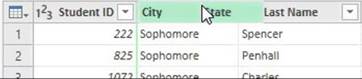
Figure14-45.SelectCityandStatecolumnheads
2.
Drag the column heads so that they are just to the right of
the Student ID column. See Figure 14-46.
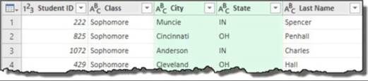
Figure14-46.DragtheCityandStatecolumnstotherightofStudentID
537
CHAPTER 14 ■ IMPORTING DATA
Closing
Query and Loading Results to Excel
1.
In the Ribbon�s Close group, click
the bottom half of the Close & Load button.
2.
Click Close & Load. See Figure 14-47.
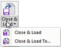
Figure 14-47. Select Close & Load
The Query Editor window
closes and the tblStudentFees and the tblStudentAddress tables are loaded into
separate worksheets. The
tblStudentAddress table is shown in Figure 14-48.
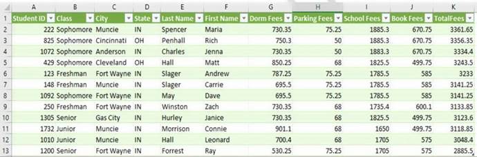
Figure14-48.Tableisloadedintoworksheet
These tables are queries. The
original data on the website has not been changed
3.
Move your cursor
over tblStudentFees in the Workbook
Queries pane. See Figure 14-49.
From this
window you can:
a.
See the last time the query was refreshed.
b.
Load the query into another
worksheet.
c.
Click EDIT which will take you back into the Query Editor.
d.
Click DELETE to delete the query.
538
CHAPTER 14 ■ IMPORTING DATA
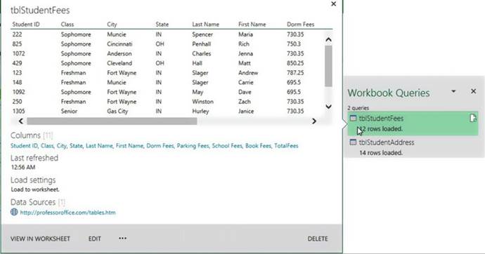
Figure14-49.tblStudentFeestable
Summary
Data can be imported into Excel from many different data sources. Once the data is imported, it can take
advantage of Excel�s wonderful analysis features.
Excel has two separate groups of command buttons for bringing data into
Excel. The two groups are Get External Data and Get & Transform. The Get External Data group buttons
bring data into a spreadsheet as is.
The Get & Transform group lets you make
modifications to the data before it is brought into your worksheet.
There are many different file types such as text files, Access files, Microsoft query files, and so on.
Different file types can use different Excel options.
Text files are files that contain no formatting, which makes it easy to import. They can be delimited or
fixed-width. The fields in a text-delimited file are separated by some character such as a comma or
semicolon. All fields have the same length in a fixed-width text file. Spaces
are added to fields to make them the same length.
The next
chapter covers Pivot Tables and Pivot Charts. A pivot table has much more
capability than a regular
Excel table. Data can be dragged into an area if you want it to be rows, and
another area if you want it to be columns, another area if you want it to be summarized. Pivot
Charts have the advantage over normal Excel charts because they can be filtered. A user can select which
items
he or she wants to appear in the Pivot Chart.
539
CHAPTER
15
Using PivotTables and PivotCharts
Few people use PivotTables
but they are missing out on probably the strongest component in Excel. It� takes a little time to learn, but
once you have conquered it, you will become an Excel power user
capable of grouping and summarizing
data in almost any form you can think of. Your boss will be amazed at what you can produce. If you are the
boss, you
will be even more amazed at yourself. PivotTables can create the types of reports managers want to see:
those
that don�t contain every detail but rather contain only the data they want to see when they want to see it.
After
reading and working
through this chapter
you should be able to
�
Create a PivotTable
�
Create a PivotChart from a data source
�
Create a PivotChart from a PivotTable
�
Rearrange and filter PivotTables
�
Create multiple PivotTables from the data source
�
Clear, move, and delete PivotTables
�
Use the slicer
tool
�
Use the time interval tool
�
Filter the data
�
Create a relational database
Working with PivotTables
It�s called a PivotTable because you can pivot your data, switching between rows and columns. You can
dynamically rearrange your existing data into an almost endless variety of different views. You can
rapidly create these views by dragging and dropping fields to different locations. Excel then automatically
recalculates the results to match the view you created.
You can create
a PivotTable from a named table or from a range of data that has not been
declared as a
table. The
benefit of creating a PivotTable from a named table is that you can take
advantage of table features such as automatically extending the table when adding rows of data.
Excel analyzes
your data and then displays �Recommended� PivotTables from which you can select
the PivotTable that matches
your needs. We will look at this feature later, but in our first practice we
will start with a simple example in
which we will create a PivotTable manually.
541
CHAPTER 15 ■ USING PIVOTTABLES AND PIVOTCHARTS
The Work & Leisure
Company is a chain of four stores
located in different areas of the country. It sells
sports products, outdoor
furniture, and tools.
The spreadsheet in Figure 15-1 shows the products the
companies sell under those categories and the number of units sold of that product during the previous month.
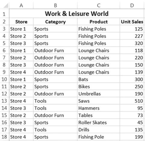
Figure15-1.DatatobeusedinPivotTable
In this exercise
you will create
a PivotTable. You will practice
rearranging the column
and row data, adding and removing fields,
changing the order
of the data, looking at different ways of summarizing the data, filtering the data, and changing the data
source
location.
1.
Open the workbook Chapter15_PivotTables.
2.
Select the worksheet named PivotTable1.
3.
Click anywhere within the data.
Click the Ribbon�s
Insert tab. In the Tables
group click the PivotTable button.
4.
The Create PivotTable dialog box displays
with a range already selected.
The range should
consist of cells $A$2:$D$18. See Figure 15-2. If this isn�t the range showing
in the text box, then change it.
5.
Change the location
of the PivotTable report to Existing
Worksheet.
542
CHAPTER 15 ■ USING PIVOTTABLES AND PIVOTCHARTS
6.
Enter F2 in the Location
text box.
7.
Click the OK button.
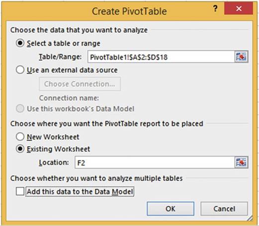
Figure15-2.SelectExistingWorksheet
8.
The PivotTable Fields list consists of five separate areas:
�
A Fields area which lists all of the column names in the
table along with a check box next to each column name
�
Filters area
�
Columns area
�
Rows area
�
Values area
9.
Click the check box for the Store field. See Figure 15-3. The store field contains
text data. Columns
that contain text are placed in the Rows area by default.
10.
Click the check box for Unit Sales.
The Unit Sales
field contains numeric
data. Columns that contain numeric
data are placed
in the Values area by default.
543
CHAPTER 15 ■ USING PIVOTTABLES AND PIVOTCHARTS
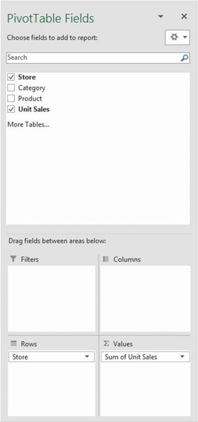
Figure15-3.SelectfieldstobeusedinPivotTable
544
CHAPTER 15 ■ USING PIVOTTABLES AND PIVOTCHARTS
The PivotTable now shows each store in its own row and it has summed all the Sales
for each one of those
stores. It also displays a grand total
that consists of all Sales from all the stores.
■
NoteYou may need to use the Zoom tool on the status bar to view all of the spreadsheet and
PivotTable at the
same time while
doing this practice.
11.
In the PivotTable Fields list, click
the check box next to Category.
Category goes to the
Rows area by default
because it contains
text. The categories
appear
as rows under their respective stores in the PivotTable. Even though the
categories are not in order in the table you are using, they are placed in their proper
order
in the PivotTable. The PivotTable now shows the total sales for each store, the
sales
for each category, and a grand total.
Hiding
and Unhiding the PivotTable Field Lists
The PivotTable Fields
list only displays when you select a cell in the PivotTable. Select a cell anywhere
outside the PivotTable and the pane disappears.
1.
Click cell A2. The pane
disappears.
2.
Click cell F2. The pane reappears.
Collapsing
and Expanding Groupings
Notice that there are minus signs to the left
of each Store. These allow you to
collapse what appears underneath a
store.
1.
Click the minus sign to the left of Store 2.
The minus
sign turns into a plus sign. See Figure 15-4
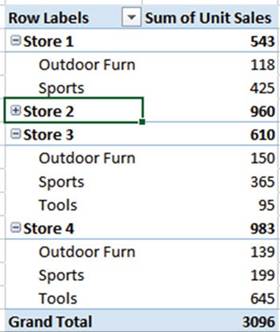
Figure
15-4.The plus and minus signs can be used to collapse and expand the
categories
545
CHAPTER 15 ■ USING PIVOTTABLES AND PIVOTCHARTS
2.
Click the plus sign to expand the details for Store 2.
Viewing Field
Values
You can view all of the different values in a field (column)
by moving your mouse over a field
in the PivotTable Fields list and then clicking the down arrow.
1.
Move your mouse over the Store field in the PivotTable Fields list. Click the down arrow to the
right of Store.
See Figure 15-5. This displays
all of the different values in the Store field.
See Figure 15-6.
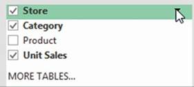
Figure15-5.ClickthedownarrowtotherightofStore
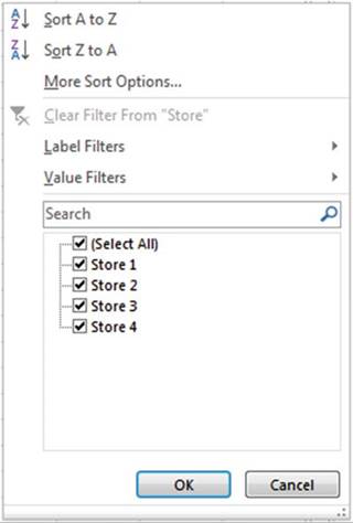
Figure 15-6.All of the different values in the Store field are displayed
2.
Click the Cancel button.
546
CHAPTER 15 ■ USING PIVOTTABLES AND PIVOTCHARTS
Filtering the
Data
1.
Move your mouse
cursor over the word Product in
the Field List.
Click the down arrow to the right
of Product. A list of all the products in the table
is displayed.
2.
Click the check boxes next to bats and bikes to remove their check marks.
3.
Click the OK button.
A filter icon appears on the line (Figure
15-7) to inform you that if you use this field, not all the items will be
displayed.
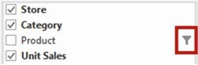
Figure 15-7.The filter icon to the right of a field informs you that the field has
been filtered
so not all the items for that field will be displayed
Because the Product
field hasn�t been placed in the PivotTable, performing a filter has no effect on what is currently displayed
in the PivotTable.
4.
Click the check box next to Product in
the PivotTable Fields list. The Products appear under their prospective categories in
the PivotTable. Widen
the columns if you need to. Notice that there are no
bats or bikes.
A Filter button
appears next to the Row Labels heading
in the PivotTable. See Figure
15-8.
5.
Move your mouse over the Filter button.
A message appears
informing you that you have manually applied
a filter to the PivotTable based on the Product field.
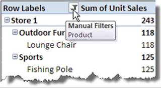
Figure15-8.AfilterbuttonappearsnexttotheRowLabelsheading
6.
Click the Filter button.
7.
Click the down arrow for the Select field and then select Product. See Figure 15-9.
547
CHAPTER 15 ■ USING PIVOTTABLES AND PIVOTCHARTS
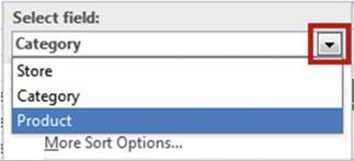
Figure 15-9. Select Product
8.
Click Clear Filter from �Product.� This
adds the bats and bikes
values to the PivotTable.
9.
Click Lounge Chairs
under Outdoor Furn in the PivotTable.
10.
Click the down arrow to the right of the Row Labels column
heading. See Figure 15-10.
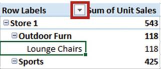
Figure15-10.ClickthedownarrowtotherightoftheRowLabelscolumnheading
11.
Since you have a product currently selected, all of the available products are listed. Click the
Cancel button.
12.
Click Outdoor Furn in the PivotTable under Store 1.
13.
Click the down arrow to the right
of the column heading Row Labels. Since you have a category
selected, all of the available categories are listed.
Click the Cancel
button.
14.
Click Store 1. Click the down arrow
to the right of the column heading
Row Labels. Since you have a store selected
all of the available stores
are listed. We only want to display
the sales for Store 2.
15.
Click the check marks next to all of the stores except for Store 2 to remove them. Click the OK
button.
The down arrow to the right of Row Labels changes to a filter icon.
16.
Bring back all of the stores by clicking the filter icon next to Row Labels.
Click the check box for Select All. (You could have accomplished the same thing by clicking
Clear Filter from �Store�). Click the OK button.
548
CHAPTER 15 ■ USING PIVOTTABLES AND PIVOTCHARTS
17.
There may
be a
large blank
area in
the PivotTable Fields list
between the
fields and the
drop areas. This
area could
prevent you
from seeing
all of
the fields
in the
drop
areas. Move your
cursor on
the dotted
line just
above the
text �Drag fields
between
areas below:�. When the
cursor changes
to a
double-headed arrow
move the mouse cursor up
to remove
some of
the space. See
Figure 15-11.
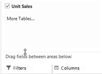
Figure 15-11.Remove
space between PivotTable Fields list and the drop areas
Changing
the Field Order
The order in which fields
are placed in the Rows drop area in the PivotTable Field
List affects the order in which they are displayed in the PivotTable. Therefore, you need to be careful
about
the order in which you drop items
into the drop area.
1.
In the Rows area drag Product
above Category. See Figure 15-12.
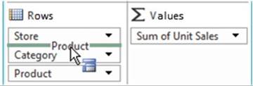
Figure15-12.DragProductaboveCategory
2.
Look at the PivotTable. Sports
now falls under bats and Outdoor Furniture
falls under Lounge Chairs. This is incorrect.
3.
Drag Category from the Rows area into
the Columns area.
The
categories are now displayed in the PivotTable as columns rather than
rows.
Notice
how the PivotTable automatically adjusted the totals.
4.
Click the down arrow to the right of Column Labels in
the PivotTable. See Figure 15-13.
549
CHAPTER 15 ■ USING PIVOTTABLES AND PIVOTCHARTS
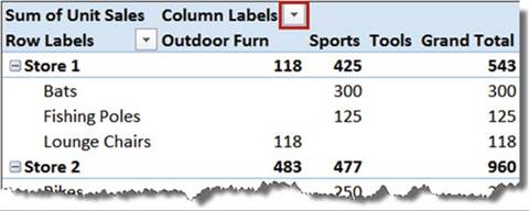
Figure15-13.ClickthedownarrowtotherightofColumnLabels
5.
Here you can filter which columns you want to display. Click
the check box next to Tools to remove it. Click the OK button.
The down arrow to the right of Column Labels
changes to a filter icon.
Removing
a Field from the PivotTable
Removing a field
from one of the drop areas of the PivotTable Fields list removes
that field from the PivotTable.
1.
Drag the Category field from the Columns drop area to the spreadsheet.
2.
As you are dragging the field over the spreadsheet, an X displays
under the field name. See Figure 15-14.
Stop dragging at this point.

Figure 15-14.As you are dragging the field over the spreadsheet, an X displays
under the field name
The Category field information is removed from the
PivotTable.
Summarizing Values
Fields in the Values area are totaled using the Sum
function. Figure 15-15 shows that Unit Sales has been summed.
550
CHAPTER 15 ■ USING PIVOTTABLES AND PIVOTCHARTS
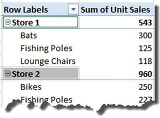
Figure15-15.ThevaluesinStore1aresummed.Thetotalis543
1.
The type of calculation can be changed
by right-clicking Sum of Unit Sales and then selecting Summarize Values By. See Figure 15-16.
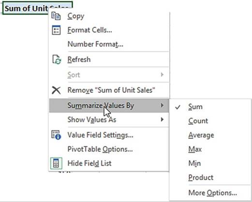
Figure 15-16.The type of calculation can be changed
by right-clicking Sum of Unit Sales and then selecting
Summarize
Values By
2.
Here in addition to the Sum
function you can elect to use
the Count, Average, Max, Min, or Product functions.
551
CHAPTER 15 ■ USING PIVOTTABLES AND PIVOTCHARTS
It would be rare that you would
use the Product function. It multiplies all the values
under a grouping. For example, in
Figure 15-15, it would determine the product of Store 1 by multiplying 300 * 125 * 118. You
can view other available functions such as variance
and standard deviation by clicking More Options�
3.
Right-click SumofUnitSalesin the PivotTable andthen select
Summarize Values By
4.
Click Average. Each of the Unit Sales is now an average
and the column
heading changed to Average of Unit Sales
5.
Try the other options.
Changing
the Data Source Location
1.
Add the records in Figure 15-17 to the spreadsheet.
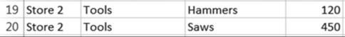
Figure15-17.Addthesetworecords
The records you added were not added to the PivotTable. Because
we selected a data range
instead of a table for our data source we will have to change
the location of our data source to include the new records.
2.
Click anywhere in the PivotTable. Click the Ribbon�s
Analyze tab, in the Data group, click the top half of the Change Data Source
button. See Figure
15-18.

Figure15-18.SelectthetophalfoftheChangeDataSourcebutton
3.
Reselect your data range so that it includes the two records
you added (don�t forget to include your column headings
in the selection). See Figure 15-19.
552
CHAPTER 15 ■ USING PIVOTTABLES AND PIVOTCHARTS
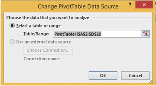
Figure 15-19.Reselect your data range
so that it includes the two records
you added
4.
Click the OK button. Your PivotTable should now include
the records you added.
In this exercise
you will look at Excel�s
recommended PivotTable formats
based on the table data you have selected.
1.
Open workbook Chapter15_PivotTables
if it isn�t opened already.
Select the worksheet named Recommended.
2.
Select the range A2:D20.
Click the Quick Analysis
button
 �at the bottom right corner of the selected
range.
�at the bottom right corner of the selected
range.
3.
Select Tables from the tabs at the top. Move your cursor over
the four recommended PivotTables. If one of them matched your needs, you could click it and Excel would
create that PivotTable on a separate
worksheet.
4.
Click the More button.
The left pane contains six recommended PivotTables. Clicking a PivotTable view in the left pane displays an
enlarged view of that PivotTable in the right pane. See Figure 15-20.
553
CHAPTER 15 ■ USING PIVOTTABLES AND PIVOTCHARTS
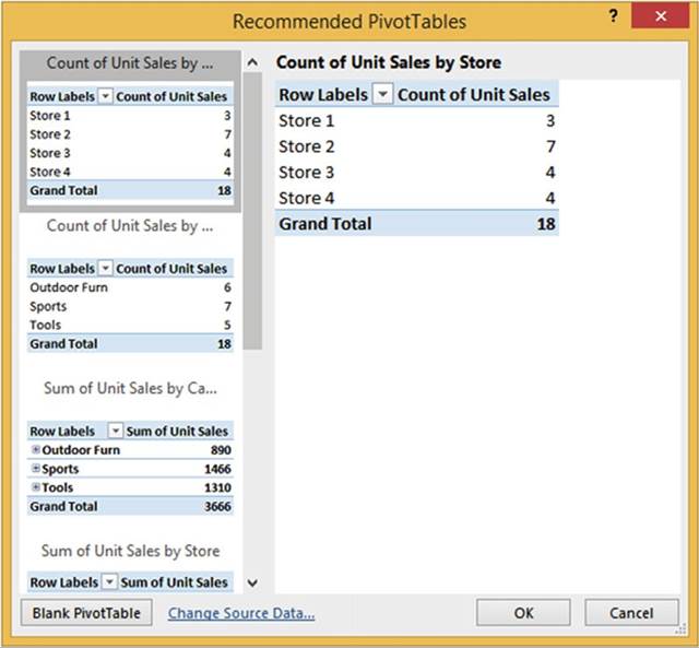
Figure 15-20.Click one of the Recommended PivotCharts in the left pane to get an
enlarged
view of it in the right pane
5.
Click the Cancel button.
6.
Click the Insert
tab on
the Ribbon. In
the
Tables group click the Recommended
PivotTables button. This brings up
the same
Recommended PivotTables dialog box that
you saw
when you
clicked the More option in
the Quick Analysis.
7.
Select the last PivotTable in the left pane. Click the OK button.
8.
The new PivotTable is created on a new worksheet.
In this exercise,
you will convert
the data from a spreadsheet into a table and then convert the table to a PivotTable. You will practice
grouping and ungrouping the fields. You will also learn how to analyze
the data by using the Slicer and TimeLine.
554
CHAPTER 15 ■ USING PIVOTTABLES AND PIVOTCHARTS
Our production line starts manufacturing radios throughout the year whenever
inventory runs low. A gauge on the line displays
the number of units produced.
An employee takes a reading
from the gauge every twenty
minutes then enters
the results into a spreadsheet. The spreadsheet covers
the years 2012 and 2013. See Figure
15-21.
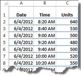
Figure 15-21. Inventory data
1.
Open the workbook Chapter15_PivotTables.
2.
Select the DateTime
worksheet.
3.
Select all the data in the Spreadsheet by doing the following:
4.
Click inside cell A1.
5.
Hold down the Ctrl + Shift keys while you press the right
arrow key and then the down arrow key.
Converting
the Data into a Table
1.
Click the Ribbon�s
Home tab and then in the Styles group click the Format
As Table button.
2.
Select the second
table in the second row of the Light category
(Table Style Light
9).
The Format As Table dialog box displays
with the selected
data for the location. See Figure 15-22.
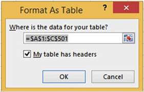
Figure 15-22. Format as Data dialog box
555
CHAPTER 15 ■ USING PIVOTTABLES AND PIVOTCHARTS
3.
Be sure that you have checked My
table has headers. Click the OK
button.
Changing
the Name of the Table
1.
Click the Ribbon�s
Design tab.
2.
In the Properties group, change
the name from Table1 to DateTimeTable.
Creating
the PivotTable
1.
Click anywhere within the data.
2.
Click the Ribbon�s Insert tab;
in the Tables group click the
PivotTable button.
3.
We will place the PivotTable on the same sheet as our data:
a.
Click the Existing Worksheet radio button.
b.
Place your cursor in the Location field.
Click cell E3. See Figure
15-23.
c.
Click the OK button.
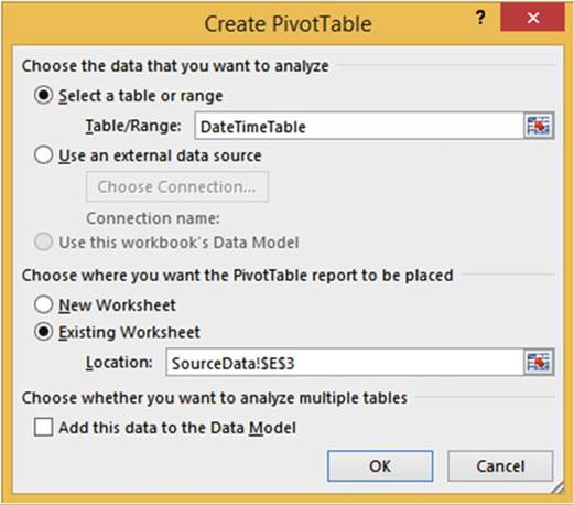
Figure15-23.ThePivotTablewillstartincellE3ofthecurrentworksheet
4.
Select Date in the PivotTable Fields list. Notice that there are two new fields
in the PivotTable Fields list that weren�t
columns in the table. Selecting a Date field adds the Quarters and Years fields
and makes them selected as well.
556
CHAPTER 15 ■ USING PIVOTTABLES AND PIVOTCHARTS
5.
Right-click 2012 in the PivotTable.
Select Expand/Collapse.
Select Expand
Entire Field.
6.
Right-click
Qtr2 under 2012 in the PivotTable. Select Expand/Collapse.
Select Expand Entire Field. You
can see that Excel breaks down (ungroups) date fields
into
years and quarters.
You can see that Excel has the intelligence
to know what months fall within what quarters
7.
Select Units in the PivotTable Fields list.
8.
Select Time
in the PivotTable fields. Notice that selecting a time field creates an Hours field which was automatically
selected. The PivotTable now shows the times in hours and the number of units
that were produced for each hour. See Figure 15-24.
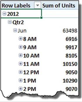
Figure 15-24.PivotTable shows the times
in hours and number of units that were produced
for each hour
9.
Click the plus sign to the left of 8 AM
to expand it. The time 8 AM
under each month expands. The 20-minute intervals display with the number
of units produced
during that time.
See Figure 15-25.
557
CHAPTER 15 ■ USING PIVOTTABLES AND PIVOTCHARTS
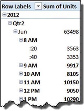
Figure15-25.Numberofunitsproducedwithin20-minuteintervals
10.
Click the minus sign to the left of 8 AM to collapse it. The time under 8 AM collapses for each
month.
11.
Right-click Qtr3 under 2012. Select
Expand/Collapse and then select Collapse
Entire Field. See Figure 15-26.
558
CHAPTER 15 ■ USING PIVOTTABLES AND PIVOTCHARTS
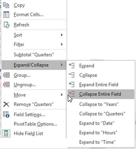
Figure15-26.SelectCollapseEntireField
12.
Click anywhere in the PivotTable. Drag Years from the Rows area
to the Columns area in the PivotTable Fields List
You can now easily compare
the number of units produced
in each quarter
of 2012 to those produced
in 2013. See Figure 15-27.
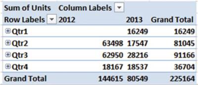
Figure15-27.Compare2012valuestothosefrom2013
13.
Click Year 2012 in the PivotTable.
559
CHAPTER 15 ■ USING PIVOTTABLES AND PIVOTCHARTS
14.
Click the Ribbon�s
Analyze tab. In the Active
Field group, click the Expand
Field button. See Figure 15-28.

Figure 15-28. Select Expand Field
15.
Click Date in the Show Detail dialog box.
See Figure 15-29.
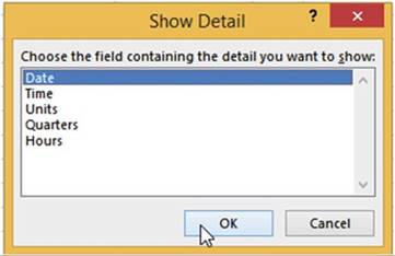
Figure 15-29. Select Date
16.
Click the OK button. Figure 15-30 shows the result.
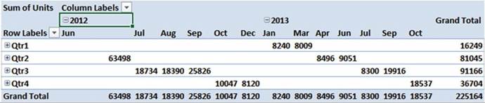
Figure15-30.YourPivotTableshouldnowlooklikethis
17.
Click Qtr1 in the PivotTable. On the Ribbons� Analyze tab, in the Active Field group,
click the Expand Field button. See Figure 15-31.
560
CHAPTER 15 ■ USING PIVOTTABLES AND PIVOTCHARTS
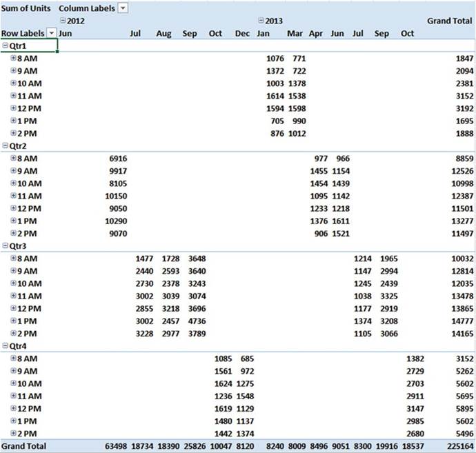
Figure 15-31. Expanded Quarter view
18.
We want to collapse the times so that we don�t see them. Click any 8 AM in the PivotTable.
Actually you can click any of the times. On the Ribbons�
Analyze tab, in the Active Field group,
click the Collapse
Field button.
19.
Drag the Years
and Date fields
from the Columns
area back to the Rows in the PivotTable Fields
pane in the order shown
in Figure 15-32.
Your
PivotTable should now look like Figure 15-33.
561
CHAPTER 15 ■ USING PIVOTTABLES AND PIVOTCHARTS
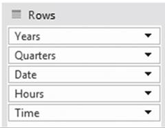
Figure 15-32. Rows pane
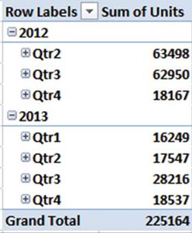
Figure15-33.YourPivotTableshouldnowlooklikethis
Grouping
and Ungrouping Fields
1.
Expand Qtr2 under 2012 by clicking the plus sign.
2.
Excel added the Years and Quarters
fields when you selected the Date field in the PivotTable Fields list. They can be removed by
using Ungroup:
a.
Click the year 2012 in the PivotTable.
b.
On the Ribbon�s Analyze tab, in group, click the Ungroup button.
The Year
and Quarter
have been
removed from the PivotTable. The
dates now
show as
they do
in the
source data. Notice that Years and Quarters
are no
longer in the Rows area.
562
CHAPTER 15 ■ USING PIVOTTABLES AND PIVOTCHARTS
3.
Click one of the times in the PivotTable
4.
On the Ribbon�s Analyze tab, in group, click the Ungroup button.
The Hours data (separated minutes) no longer
appears in the PivotTable. The Time now shows
as it does in the source data. Notice
that Hours is no longer in the Rows area.
5.
Click the Ribbon Design tab. In the Layout group click the Report Layout button. See Figure
15-34.
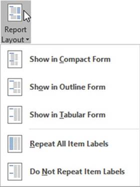
Figure15-34.OptionsunderReportLayoutbutton
The PivotTable is currently displayed in the Compact Form.
6.
Click Show in Outline
Form. The Outline
Form separates the Date and Time field into separate
columns. The Sum of Units displays at the top of the data being summed.
7.
Click the Report Layout button
again. Click Show in Tabular Form.
The first Time and Units appear on the same row as the Date. The total of the Units appears
at the end of each Date rather than at the top. Figure 15-35 shows how each of the Report Layout types
treats the same data.
563
CHAPTER 15 ■ USING PIVOTTABLES AND PIVOTCHARTS
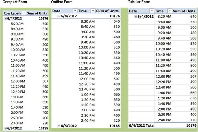
Figure15-35.Threetypesofforms:Compact,Outline,andTabular
Notice the Compact
Form doesn�t display
a separate Date column as do the Outline and Tabular forms.
8.
Click the Report
Layout button and then click Repeat
All Item Labels. See Figure 15-36
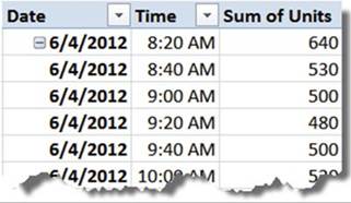
Figure15-36.Datesarerepeateddownthecolumn
564
CHAPTER 15 ■ USING PIVOTTABLES AND PIVOTCHARTS
9.
Remove the repeated dates by clicking the Report Layout button and then
clicking
Do Not Repeat Item Labels.
10.
On the Ribbon�s Design tab, in
the Layout group, click the Subtotals
button. Select
Do Not Show Subtotals. The Subtotals
are removed from the PivotTable.
11.
Click the Subtotals button again. Select
Show all Subtotals at Bottom of Group. The subtotals appear
at the bottom of each date.
12.
On the Ribbon�s Design tab, in
the Layout group, click the Blank
Rows button.
13.
Select Insert Blank Line after Each
Item. A blank line appears
between each date
14.
Click the date 6/4/2012 in the PivotTable.
15.
Click the Ribbon�s Analyze tab. In the Active Field group, click the Collapse Field
button.
16.
Click the Ribbon�s Design tab, in
the Layout group, click the Blank
Rows button.
17.
Select Remove
Blank Line after Each Item.
18.
On the Ribbon�s
Design tab, in the PivotTable Styles group, click
one of the styles you like.
Adding Records to the Source Data and Refreshing the
PivotTable
When you add new
records,
the
PivotTable doesn�t automatically update to reflect the new records. The data source doesn�t
need to change since we are using a table; however, the PivotTable still needs to be
refreshed.
1.
Add the three records in Figure 15-37 to the bottom of the source data.
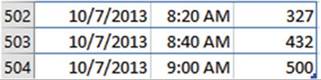
Figure 15-37. Add this data
2.
Click any cell in the PivotTable. Click the Ribbon�s
Analyze tab. In the Data group, click the top half of the Refresh
button.
The records you added should now appear at the bottom of the PivotTable. See Figure 15-38.
565
CHAPTER 15 ■ USING PIVOTTABLES AND PIVOTCHARTS
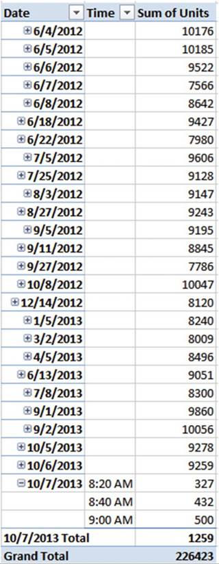
Figure15-38.RecordsyouaddedappearatthebottomofthePivotTable
566
CHAPTER 15 ■ USING PIVOTTABLES AND PIVOTCHARTS
3.
Click the minus sign next to 10/7/2013.
4.
Click the Ribbon�s Analyze tab. In the Filter group, click Insert Slicer.
5.
Check Date and Time. Click the OK button.
6.
Click 6/6/2012 in the Date slicer. Only the data for that date displays.
If you want to select
more than one date at a time you will need to click the multi-select button on the top right of the slicer.
See Figure 15-39.
Click on the date in the Pivot Table.
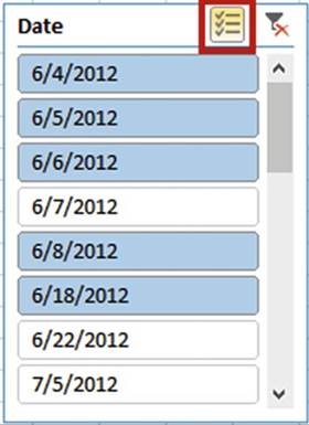
Figure 15-39. Date slicer
■
Note� If you click an item in the slicer and then click
multi-select, all other
items become unselected and then you click the rest of the items
you need. If you haven�t
clicked on an item before
you click multi-select, then items you click actually
become deselected.
7.
Click the Ribbon�s
Analyze tab. In the Active
Field group, click
the Expand Field button.
8.
Click the Clear filter button for the Date slicer.
9.
Click 6/4/2012 in the Date slicer. The
other dates are no longer selected.
10.
Click the multi-select button.
11.
Select the other four dates shown in Figure 15-39.
12.
Click 10:00 AM in
the Time slicer. Click the multi-select button. Select times 10:20 AM, 10:40 AM, and 11:00
AM. See Figure 15-40.
567
CHAPTER 15 ■ USING PIVOTTABLES AND PIVOTCHARTS
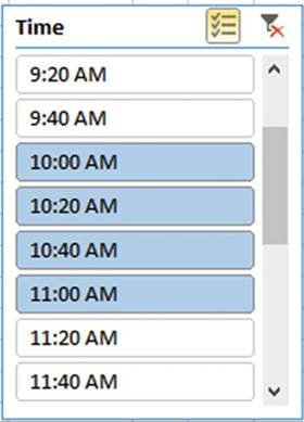
Figure 15-40. Time Slicer
13.
Click anywhere on the PivotTable. Click the Ribbon�s
Analyze tab. In the Filter
group, Click Insert
Timeline.
14.
Check Date. Click the OK button.
15.
The Time line has
a horizontal scroll bar. Scroll all
the way to the left. Under 2012 click
June.
16.
All the June 2012 dates display in the PivotTable. Drag across June,
July, and August.
See Figure 15-41.
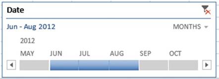
Figure 15-41. Time line
All the June, July, and August dates appear in the PivotTable.
568
CHAPTER 15 ■ USING PIVOTTABLES AND PIVOTCHARTS
You have
learned how to create PivotTables. You have seen that you can move fields to
different areas in the
PivotTable Fields pane to control rows, columns, and summarizing. You have also
seen how easy it is easy to view only data from a particular time or
date using a slicer or a time line. Next, you will learn how to create a
chart that can be filtered.
Creating a PivotChart
PivotCharts can be created
directly from a data source or from a PivotTable. The difference between a PivotChart
and other charts is that a PivotChart has filter buttons associated with it
that the user can use to view just what he or she wants on the chart.
In this exercise, we first will create a PivotChart from a data source. Then we will create one from a
PivotTable.
1.
Open the Chapter15_PivotTables workbook.
2.
Select the worksheet named PivotChart.
Creating a
PivotChart based on Source Data
1.
Click anywhere within
the data. Click
the Ribbon�s Home tab. In the Styles
group, click Format
As Table.
2.
Select the second style in the second row (Table Style Light 9).
3.
Click the Ok button for Format As Table.
See Figure 15-42.
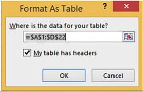
Figure15-42.FormatAsTabledialogbox
4.
Click the Ribbon�s
Insert tab. In the Charts
group, click the top half of the PivotChart button.
The Create PivotChart dialog box displays.
5.
Select Existing Worksheet. Click inside the Location text box. Click
inside cell F2. See Figure 15-43.
569
CHAPTER 15 ■ USING PIVOTTABLES AND PIVOTCHARTS
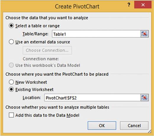
Figure 15-43. Create PivotChart dialog box
6.
Click the OK button.
7.
You create a
PivotChart the same way that
you create
a PivotTable.
Select State, Category, Product, and Sales in
the PivotChart
Fields list.
8.
Expand the size of the chart so that you can see everything. There are three filter buttons below
the chart. See Figure 15-44.

Figure 15-44. Filter buttons
570
CHAPTER 15 ■ USING PIVOTTABLES AND PIVOTCHARTS
9.
Click the State
filter button. Remove
the check in front of Illinois. Click
the OK button. Now just the data for Indiana and Kentucky shows.
10.
Click the Category filter button. Remove the check in front of books _Mag. Click the OK button.
11.
Click the Product
filter button. Remove the check in front of Beverages. Click the OK button. Your PivotChart should look like
Figure 15-45.
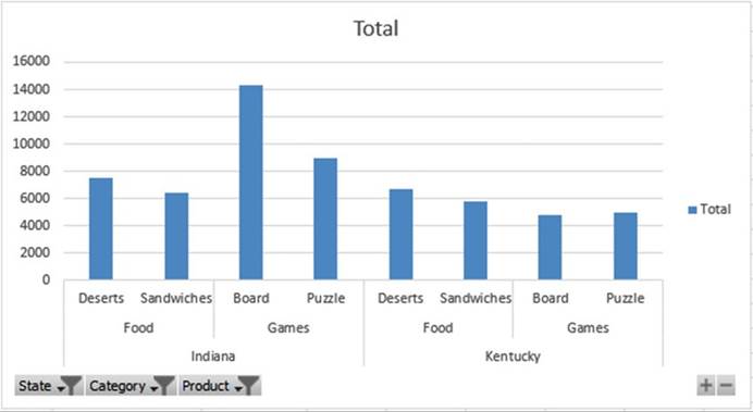
Figure15-45.YourPivotChartshouldnowlooklikethis
12.
Click the State filter button. Select Clear
Filter from �State.�
13.
Click the Category filter button. Select
Clear Filter from �Category.�
14.
Click the Product filter button. Select
Clear Filter from �Product.�
■
Note� When you created a PivotChart, a PivotTable was created
at the same time. When
you make changes to the PivotChart, the same changes are made to the PivotTable.
Below the chart on the right
there is a plus and minus button.
The plus button
is the Expand Entire Field
button. The minus
button is the Collapse Entire
Field button.
15.
Click the minus button. This
collapses all of the Product data. See
Figure 15-46.
571
CHAPTER 15 ■ USING PIVOTTABLES AND PIVOTCHARTS
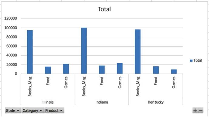
Figure15-46.Productdatahasbeenremoved
16.
Click the plus button. This
brings back all of the Products.
17.
Press the Delete key to remove the PivotChart.
18.
Click anywhere in the PivotTable. Click the Ribbon�s
Analyze tab. In the Actions
group, click the Select button.
19.
Select Entire PivotTable. Press the Delete key.
Creating
a PivotChart Based on a PivotTable
1.
Click anywhere in the table data. Click
the Ribbon�s Insert tab.
2.
In the Tables group, click PivotTable. The Create PivotTable dialog box displays.
3.
Select Existing Worksheet. Click inside the Location text box. Click inside cell F2.
4.
Click the OK button.
5.
Select the State,
Category, Product, and Sales fields in the PivotChart Fields list
6.
Move the Category
and Product fields from the Rows area to the Columns area. See Figure 15-47.
572
CHAPTER 15 ■ USING PIVOTTABLES AND PIVOTCHARTS
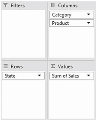
Figure15-47.MovedCategoryandProducttotheColumnsarea
The PivotTable should look like Figure 15-48.
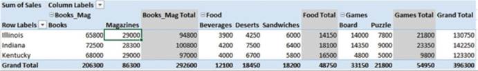
Figure15-48.YourPivotTableshouldnowlooklikethis
7.
Click anywhere on the PivotTable. Click the Ribbon�s Analyze button. In the Tools group, click the
PivotChart
button.
The Insert Chart dialog box displays. See
Figure 15-49.
573
CHAPTER 15 ■ USING PIVOTTABLES AND PIVOTCHARTS
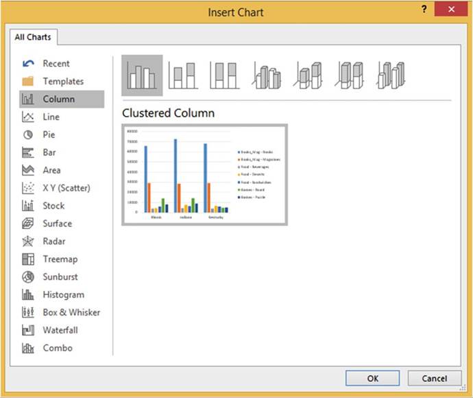
Figure 15-49. Clustered Column chart
8.
Leave the Clustered Column chart selected. Click the OK button.
9.
The PivotChart displays.
See Figure 15-50.
It is based on the PivotTable. It takes on the same format. The results here are much different than the
first PivotChart you created from the source
data.
574
CHAPTER 15 ■ USING PIVOTTABLES AND PIVOTCHARTS
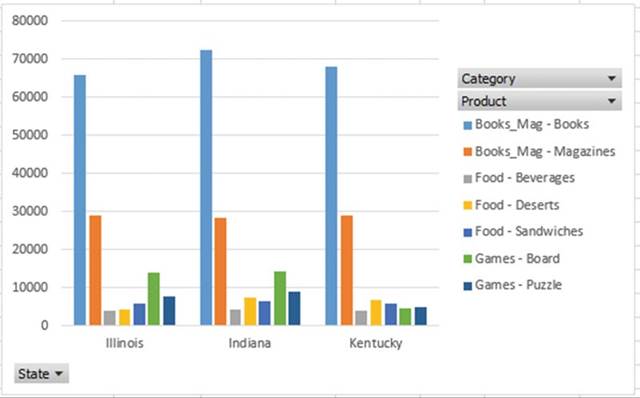
Figure 15-50. PivotChart
Creating Multiple PivotTables and PivotCharts from the
Same Data Source
It is possible
to create multiple
PivotTables with different
structures from the same data source. You may want to create multiple PivotTables so you can look at various
summarized views of your data at the same time.
1.
Click anywhere in the source data.
2.
Bring up the PivotTable and PivotChart Wizard by pressing the Alt key, then the D key, and then
the P key. (Do not press any of
them at the same time.) If you are not at Step 1 of 3 of the Wizard, press the Back button
until you are.
3.
Leave Microsoft
Excel list or database selected.
Select PivotChart report
(with PivotTable report). See Figure 15-51.
Click the Next button.
575
CHAPTER 15 ■ USING PIVOTTABLES AND PIVOTCHARTS
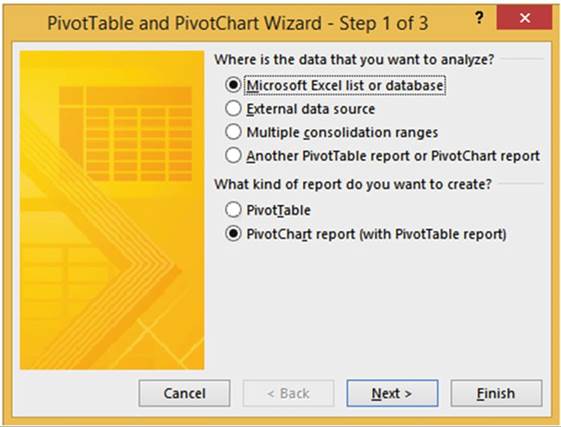
Figure15-51.PivotTableandPivotChartWizard�Step1of3
4.
Step 2 of the Wizard should
have the range as shown in Figure 15-52.
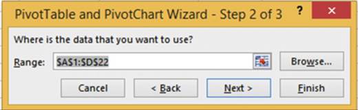
Figure15-52.PivotTableandPivotChartWizard�Step2of3
5.
Click the Next button.
6.
Select Existing worksheet. Click in cell F35. See Figure 15-53.
576
CHAPTER 15 ■ USING PIVOTTABLES AND PIVOTCHARTS
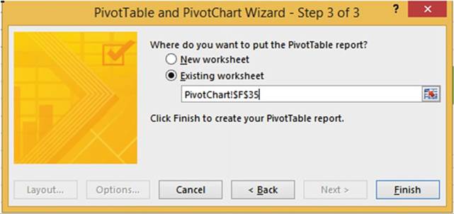
Figure15-53.PivotTableandPivotChartWizard�Step3of3
7.
Click the Finish button.
8.
In the PivotTable Fields list select the State, Category, and Sales fields.
9.
Drag the State field from the Axis (Categories) area to the Legend (Series)
area.
10.
Close the PivotChart Fields list.
The
PivotTable should now look like Figure 15-54.
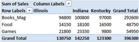
Figure15-54.YourPivotTableshouldnowlooklikethis
The PivotChart should now look like Figure 15-55,
577
CHAPTER 15 ■ USING PIVOTTABLES AND PIVOTCHARTS
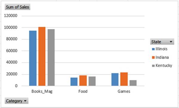
Figure15-55.YourPivotChartshouldnowlooklikethis
Moving
the PivotChart and PivotTable
You move the
PivotChart by moving the cursor
to its
border. The
cursor changes to a four-headed
arrow. Drag the PivotChart to
wherever you want. There are two ways
to move
a PivotTable. You can use drag and
drop if
you are
moving the PivotTable to another
location on the same worksheet
or you
can use
the Move
PivotTable button on the Ribbon.
1.
Click the PivotTable you just created.
2.
On the Ribbon, click the Analyze Tab. In the Actions group click the Select button
and then select Entire PivotTable. See Figure 15-56.
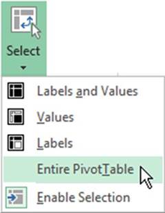
Figure15-56.SelectEntirePivotTablefromtheSelectbutton
578
CHAPTER 15 ■ USING PIVOTTABLES AND PIVOTCHARTS
3.
Move the cursor to any border of the PivotTable. The cursor changes
to a four-headed arrow to signify that the PivotTable is now able to be dragged.
4.
Drag the PivotTable so that it starts in cell G33. You may need to widen the columns.
5.
Relocate the PivotTable
using the
Move PivotTable
button. 6. Click
anywhere on the PivotTable.
On the Analyze tab
in the Actions
group click
the Move
PivotTable button. The Move Table dialog
box displays. With the cursor in the
Location textbox click cell D34. Click
the OK
button.
Clearing a
PivotTable
1.
In the Ribbon�s Action group, click the Clear button.
2.
Select Clear All. This
clears all the data and labels but the PivotTable still exists.
Deleting a
PivotTable
1.
Press Ctrl + Z to undo the Clear
2.
Click inside any cell in the PivotTable
3.
In the Actions group click the
Select button. Select Entire
PivotTable.
4.
Press the Delete key.
Deleting a
PivotChart
1.
Click the PivotChart.
2.
Press the Delete key.
You have learned how to create a PivotChart from source data and from a PivotTable. You have learned how to
create different PivotTables from the same data source and how to use the PivotTable and PivotChart Wizard.
Next,
you will learn
how you can take data from different sources and link them together
by a key field.
Creating PivotTable on a Relational Database
PivotTables become even more powerful when you can apply them to multiple files that are linked together.
You can do this through a relational database.
When we think
of databases we usually think of programs such as Access, SQL Server, Oracle,
and so on. We can import data from
these programs into Excel. We can, however, create small relational databases directly in Excel. A
relational
database is created by linking multiple tables through a common field. The tables can be linked together to
create a PivotTable.
Relational
databases consist of Master and Detail tables. If you have previously used
Access you are
probably
familiar with the concept. There must be a common field in the master and
detail files on which the
tables are linked together. There is one Master record for one or more detail
records.
Figure 15-57 shows a Customer table and 15-18 shows an Orders table. The two tables can be linked by the
common field CustomerID. Each customer in the Customer table is assigned a unique CustomerID. Each customer
can make many orders; therefore, the CustomerID field in the Orders table is not unique. We call this type
of relationship between the two tables a one-to-many relationship. The fields used to link tables are called
keys. The common field that is unique is called the PrimaryKey. The common field on the
many side is called the ForeignKey. Looking at the two tables you can see that a CustomerID
must already exist in the Customer table before it can be used in the Orders table.
579
CHAPTER 15 ■ USING PIVOTTABLES AND PIVOTCHARTS
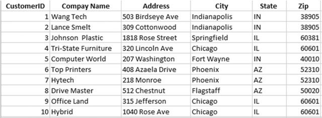
Figure 15-57. Customer table
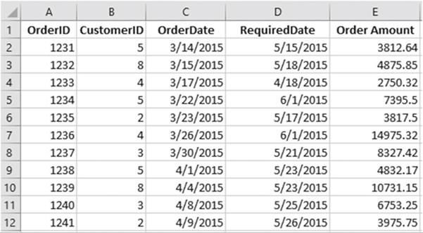
Figure 15-58. Orders Table
In this exercise
you will first
create the Master
table and then the Detail
table. You will then link the two tables together. You will then create a PivotTable that uses the two
linked
tables.
580
CHAPTER 15 ■ USING PIVOTTABLES AND PIVOTCHARTS
Creating
the Master Table
1.
Open the Chapter15_PivotTables workbook. Select the worksheet named Master. Click anywhere in the
data.
2.
Click the Ribbon�s
Home tab. In the Styles group, click the Format as Style button. Select
any style you wish.
The Format As Table dialog box displays. See Figure 15-59.

Figure15-59.FormatAsTabledialogbox
3.
Be sure that you select My table
has headers and then click the OK button.
4.
The Design tab is active when you
select the table.
In the
Properties group,
change
the Table Name to Customer and then press Enter.
Creating
the Detail Table
1.
Click the worksheet tab named Detail. Click anywhere in the data.
2.
Click the Ribbon�s
Home tab. In the Styles group, click the Format as Style button. Select
any style you wish.
3.
Be sure that you select My table has headers in the Format
As Table dialog box and then click the OK button.
4.
The Design tab is active when you
select the table. In the
Properties group, change
the Table Name to Orders and then press Enter.
Linking the
Tables Together
1.
Click the Ribbon�s
Data tab. In the Data Tools group,
click the Relationships button.
2.
Click the New button. See Figure 15-60.
581
CHAPTER 15 ■ USING PIVOTTABLES AND PIVOTCHARTS
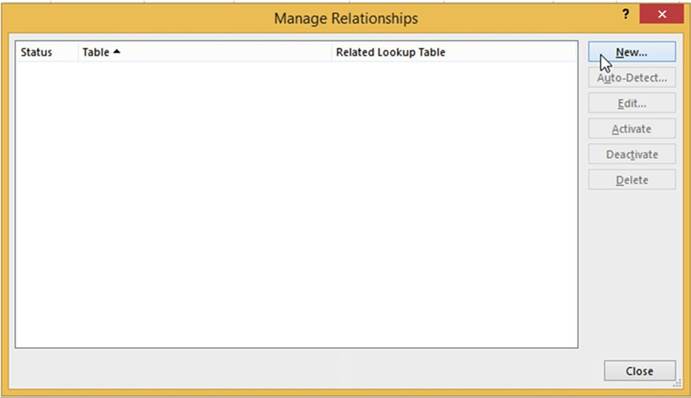
Figure15-60.ManageRelationshipsdialogbox
3.
The Customer table and the Orders
table both contain a CustomerID field by which they can be linked together. The CustomerID field in
the customer table is the Primary key and the CustomerID in the Orders table is
the Foreign key. Make
the entries shown in Figure 15-61 and then click the OK button.
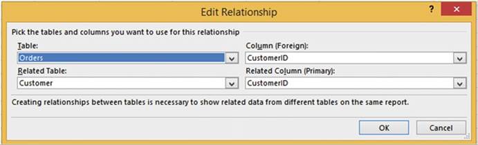
Figure15-61.EditRelationshipdialogbox
582
CHAPTER 15 ■ USING PIVOTTABLES AND PIVOTCHARTS
4.
The Manage Relationships dialog box shows the relationship you just created.
Click the Manage
Relationships Close button.
See Figure 15-62.
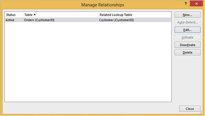
Figure 15-62.Relationship you created between Orders
and Customer
Defining
the Table Relationships in the PivotTable Report Section
1.
Click the Ribbon�s
Insert tab. In the Tables group, click the PivotTable button. The Create
PivotTable dialog box displays. See Figure 15-63. The Table/Range
should be Orders.
2.
For the option
Choose whether you want to analyze
multiple tables, select Add this data to the Data Model.
3.
Click the OK button.
583
CHAPTER 15 ■ USING PIVOTTABLES AND PIVOTCHARTS
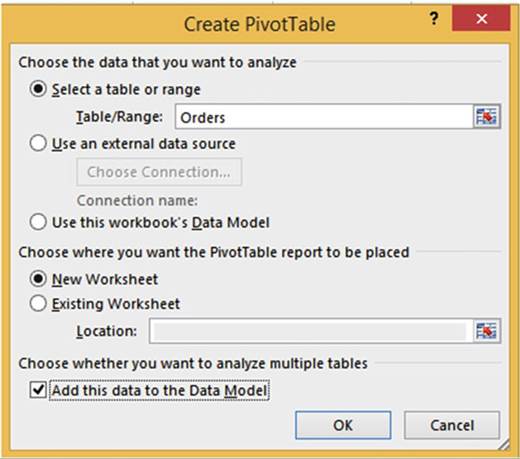
Figure15-63.CreatePivotTabledialogbox
4.
In the PivotTable Fields list on the right side of the worksheet, the word Active is
highlighted. The word Active is
highlighted because there is only one table currently active.
Click the word All.
See Figure 15-64.
Expand the Customer
and Orders tables
so that you can see all of their fields.
584
CHAPTER 15 ■ USING PIVOTTABLES AND PIVOTCHARTS
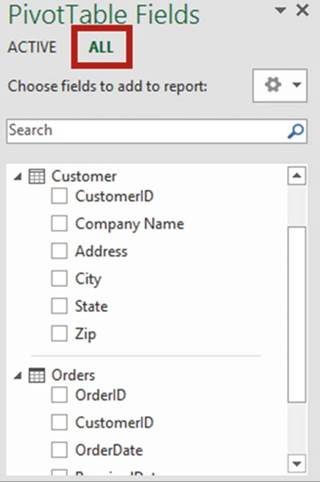
Figure15-64.ClickthewordAlltoseeallofthefieldsforbothtables
We have already
created the relationship between the tables,
but if we hadn�t and you start
adding fields in the PivotTables that can�t be made sense
of without the relationship, you will get the message
in Figure 15-65.
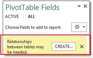
Figure15-65.Possiblemessage
585
CHAPTER 15 ■ USING PIVOTTABLES AND PIVOTCHARTS
Clicking the CREATE button
would bring up the same Create Relationship dialog box that you already filled
out.
5.
Now you can create a PivotTable using
both tables. In the
PivotTable Fields pane, select the fields CustomerID, City, and State from the Customer table.
6.
Select the fields
OrderID and Order
Amount from the Orders table.
The bottom half of the PivotTable Fields
list appears as in Figure
15-66.
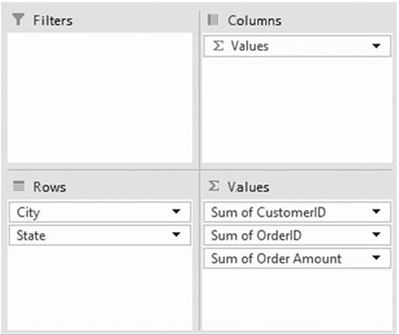
Figure15-66.Yourareasshouldlooklikethis
586
CHAPTER 15 ■ USING PIVOTTABLES AND PIVOTCHARTS
7.
Now, let�s rearrange the fields:
a.
Drag State from the Rows area to the Filters area.
b.
Drag Sum of CustomerID from Values
to the top of Rows.
c.
Drag Sum of OrderID from Values to the bottom of Rows. The areas should look like Figure 15-67.
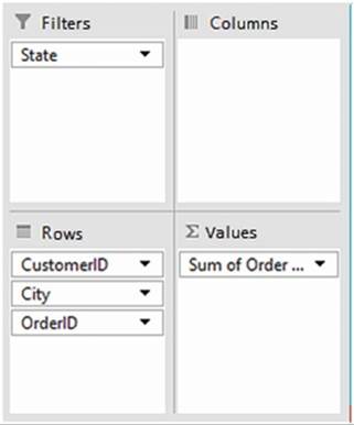
Figure15-67.Yourareasshouldlooklikethis
587
CHAPTER 15 ■ USING PIVOTTABLES AND PIVOTCHARTS
The
resulting PivotTable should
look like Figure
15-68.
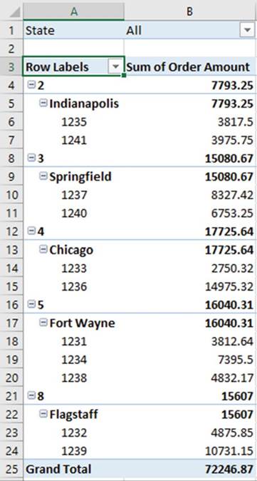
Figure15-68.YourPivotTableshouldlooklikethis

588
Summary
CHAPTER 15 ■ USING PIVOTTABLES AND PIVOTCHARTS
PivotTables provide you with extreme flexibility in what data is to be displayed, how it is to be arranged,
and what values you want summarized. It�s called a PivotTable because you can pivot your data, switching
between rows and columns.
PivotCharts have the advantage over other charts in that they can be filtered. Small relational databases can
be created directly in Excel.
The next chapter deals with using Multimedia in a workbook. Multimedia is using different forms of
communication. You will use different forms of text, diagrams, pictures, screen captures, audio, and video
to communicate in a workbook.
589
CHAPTER
16
Enhancing
Workbooks with Multimedia
Multimedia includes all the different types of media.
You have been using text media, but you can add images,
shapes, clipart, videos,
and audio to your spreadsheets. Multimedia can help you capture
your audience�s attention by increasing the appeal of your spreadsheets. SmartArt provides a variety of
organizational and other charts
that you can alter to fit your needs. You can grab a screen
capture from a web site or an Excel example
and then place
that capture in the current
worksheet.
After reading and
working through this chapter you should be able to
�
Add and edit images
�
Use WordArt
�
Add and change shapes
�
Grab an entire window or a portion of it and
make it an image
�
Use SmartArt
�
Add video
�
Use audio
Adding Pictures
to the Worksheet
You can add pictures to your worksheet
from either your computer or the Internet.
There are two buttons in the Insert tab�s Illustrations group for accessing
pictures. The Pictures
button is for getting pictures
from your computer and the Online Pictures button is for getting pictures
from the Internet.
See Figure 16-1.
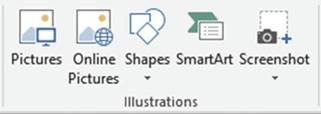
Figure16-1.Ribbon�sIllustrationsgroup
591
CHAPTER 16 ■ ENHANCING WORKBOOKS WITH MULTIMEDIA
If you click the Pictures button
Excel will display
the Insert Picture
dialog box from where you can browse to locate
images on any drives directly
connected to your computer or through a network.
If you click the Online Pictures
button, Excel will display the Insert Picture
window for online
pictures. See Figure
16-2. The window
provides you with four locations for downloading images
from the Internet:
�
Microsoft�s Bing search engine
�
OneDrive
�
Facebook
�
Flickr
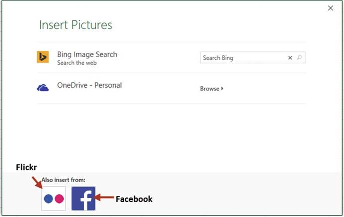
Figure 16-2. Insert Picture
window
Flickr is a social media
web site that lets users
upload pictures and share them.
Enter your search word or phrase
into the Bing Image Search
text box. Images
matching your search word or phrase are displayed. Dog was entered for the search
word in Figure
16-3. A message
may appear saying
that the images
are licensed under
Create Commons. To get other
images click the Show all web results
button. Click
an image and then click
the Insert button
to paste it into your worksheet.
592
CHAPTER 16 ■ ENHANCING WORKBOOKS WITH MULTIMEDIA
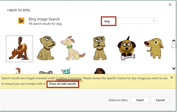
Figure16-3.Theworddogwasenteredforthesearch
In this exercise you will explore various
ways of altering images, adding
borders to an image and applying
picture styles.
1.
Open Workbook Chapter 16. Create a new worksheet.
2.
Click the Ribbon�s Insert tab. In
the Illustrations group, click
Pictures.
3.
Browse to the Chapter 16 folder. Locate the Pilot picture. Figure 16-4 shows
the picture.
593
CHAPTER 16 ■ ENHANCING WORKBOOKS WITH MULTIMEDIA

Figure 16-4. Pilot picture
4.
When you have an image selected on
your worksheet the Ribbon will have a Format tab. The Format tab has all the options for
altering, sizing, coloring, rotating, cropping, applying effects, adding borders, and so on, to your image.
Click the Image. Click the Ribbon�s
Format tab.
5.
In the Adjust group, click Corrections. The corrections gallery
shows thumbnails of your image with various levels of sharpness, brightness, and contrast. See
Figure 16-5. The image in the center of the Sharpen/Soften group and in the
center of the Brightness/Contrast group has a border around it. The images with borders
around
them represent the way your image looks currently. Move your cursor over
the thumbnails
while observing the effects they have on the selected image on the
worksheet.
As you move farther to the right in the Brightness/Contrast group the
brightness increases. As you move farther down in the group the contrast increases.
If you want to apply one of the effects to your selected image, click the thumbnail.
If you decide you don�t like the effect, you can undo it by pressing Ctrl + Z.
594
CHAPTER 16 ■ ENHANCING WORKBOOKS WITH MULTIMEDIA

Figure 16-5.Corrections gallery where you can vary the level of sharpness,
brightness, and contrast
In the Adjust group there is a Reset Picture
button that lets you reset
either just the picture or both the picture and its size back to the way it was when you inserted it.
6.
In the Adjust
group, click the Color button.
See Figure 16-6. The adjustments here affect the saturation, tone,
and overall color of the image. Move your cursor over the thumbnails while observing the effects they have
on the selected
image on the worksheet.
595
CHAPTER 16 ■ ENHANCING WORKBOOKS WITH MULTIMEDIA
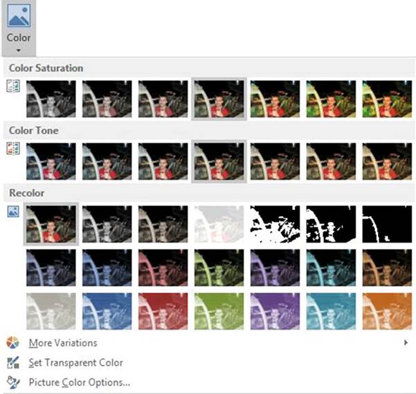
Figure16-6.Adjustoverallcolor,saturation,andtoneoftheimage
7.
In the Adjust
group, click the Artistic Effects
button. Move your cursor over the thumbnails while observing the effects they have on the selected
image on the worksheet. Figure
16-7 shows the special effects,
pencil sketch and photocopy, applied
to the image.
596
CHAPTER 16 ■ ENHANCING WORKBOOKS WITH MULTIMEDIA

Figure16-7.Specialeffects:pencilsketchandphotocopy
8.
The best way to create a dramatic
effect without altering
the appearance of your picture
is to use one of the styles from the Picture Styles Gallery. See Figure 16-8.
Figure16-8.PictureStylesGallery
9.
Move your cursor over the styles while observing the
effects they have on the selected
image on the worksheet.
Figure 16-9 shows some of the various ways that Picture Styles can
display your image.
597
CHAPTER 16 ■ ENHANCING WORKBOOKS WITH MULTIMEDIA

Figure 16-9.Various ways that Picture
Styles can display
your image
10.
In the Picture
Styles group, click
the down arrow for Picture
Border. Select a red color and change the weight of the border to 3 pt. See Figure
16-10.

Figure16-10.Redborderwithweightof3pt
598
CHAPTER 16 ■ ENHANCING WORKBOOKS WITH MULTIMEDIA
11.
Click Picture Effects.
There are seven groups of various effects.
Move your cursor over the various Picture
Effects while observing
their effect on the selected
image on the worksheet. The picture in Figure 16-11 has a glow effect.

Figure 16-11. Glow effect
You have learned
how to add images to your worksheet from your saved
image files on your computer.
What if you wanted to add an image that you see on a web site or what if you wanted to write training
documentation and needed
an image from Excel or Word or some other
application? Excel has a feature
called Screenshot that allows you to grab those images.
Using Screenshot
Use Screenshot to grab an entire window
or a portion of it and turn it into an image.
The Screenshot button
is located on the Insert
tab in the Illustrations group.
Clicking the Screenshot button opens a thumbnail view of
all available windows.
See Figure 16-12. Clicking
one of these thumbnails captures
a full size image of that
window.
599
CHAPTER 16 ■ ENHANCING WORKBOOKS WITH MULTIMEDIA
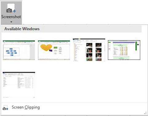
Figure 16-12.Screenshot can capture one of the open
windows on your computer
If you only want to grab a portion
of a window, you will need to open that window prior
to clicking Screen
Clipping. After clicking
Screen Clipping, the Excel program
minimizes, the window
that you are capturing from dims, and the cursor
turns into a crosshair. As you drag your mouse,
the area that will be included in your image
brightens. When you have finished
selecting the area you want,
the image appears
in your worksheet.
In this exercise you will grab a portion of a
web site which will then be stored in your worksheet. You will apply a
picture style to the captured image.
1.
Click the Screenshot Worksheet
2.
Close or minimize all open windows except Excel.
3.
Click the hyperlink in cell A1
4.
Scroll down on the web page until the entire Income
Statement shown in Figure 16-13
is visible.
600
CHAPTER 16 ■ ENHANCING WORKBOOKS WITH MULTIMEDIA
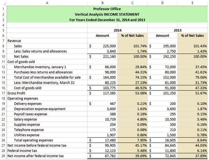
Figure16-13.WindowthatwillbecapturedwithScreenshot
5.
If the web page is maximized, change
the size of the window so that you can see the Income Statement
in your web browser and the Insert tab in Excel at the same time.
6.
Click the Ribbon�s Insert tab. In
the Illustrations group, click the
Screenshot button.
7.
Click Screen Clipping at the bottom of the window. The Excel program becomes hidden while getting
the screen clipping.
8.
Using the crosshair, drag across the income statement. As you drag across the income statement the
area that will be included in the captured
image becomes highlighted. See Figure 16-14. When you release
the mouse, the highlighted area becomes an image that is stored on your worksheet.
601
CHAPTER 16 ■ ENHANCING WORKBOOKS WITH MULTIMEDIA
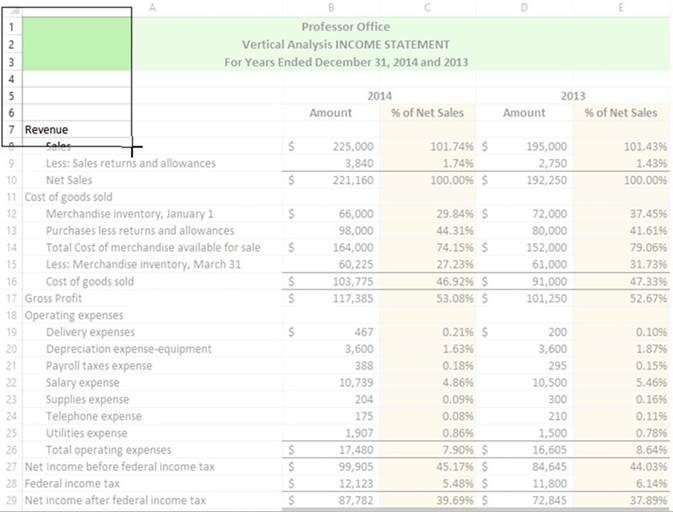
Figure 16-14.As you drag across the income statement
the area that will be included in the captured
image becomes highlighted
The screen clipping is an image and therefore
all the functions that can be applied to
an image can be applied to the screen clipping.
9.
Maximize your Excel window. Move your spreadsheet image to the center of your worksheet window.
10.
Click the Ribbon�s
Format tab. In the Picture�s Styles group, select
Drop Shadow Rectangle from
the Styles gallery.
This will add a shadow to the bottom and right side of the image.
602
Working with
WordArt
CHAPTER 16 ■ ENHANCING WORKBOOKS WITH MULTIMEDIA
WordArt is decorative text that you have far more control
over than the normal text. You can warp WordArt text, make it follow a path, change its shape, give it a 3-D
look, change its font, change its background, etc.
In this exercise you will explore various ways of creating and altering WordArt.Create a new worksheet.
1.
Click the Ribbon�s
Insert tab. In the Text group, click
the WordArt button.
See Figure 16-15.

Figure 16-15. WordArt
2.
Select the first A in the first
row.
3.
Type Happy Note Music. Select
the text.
WordArt uses the font type that is selected in the Font
group on the Home tab.
4.
Click the Ribbon�s
Home tab, and in the Font group,
click the down arrow for the Font Type. Move your cursor over the font types as you watch its effect on your
WordArt.
5.
Click the Ribbon�s
Format tab. In the WordArt
Styles group click
the down arrow
for Text Fill.
See Figure 16-16.
603
CHAPTER 16 ■ ENHANCING WORKBOOKS WITH MULTIMEDIA
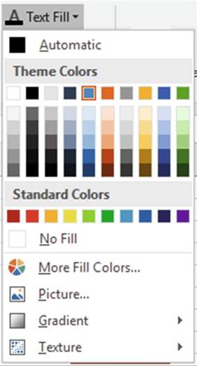
Figure 16-16. Text Fill options
6.
Move your cursor over the different colors to see the effect on your WordArt.
7.
Click Texture. Move your cursor
over each of the Textures
to see the effect on your WordArt.
8.
Notice that you can even fill your text with a Picture.
9.
The Gradient depends
upon the color
that you are currently using.
We won�t make any changes.
10.
In the WordArt
Styles group click the down arrow for Text Outline.
You can pick a color for the outline and then change
the size of the outline
by changing the weight. Select
green for the color. Click back on the down arrow for Text Outline
and select a weight of 1 pt.
11.
In the WordArt Styles group click Text Effects. Go through the Shadow, Reflection, and Glow
options as you observe their effect on the WordArt.
604
CHAPTER 16 ■ ENHANCING WORKBOOKS WITH MULTIMEDIA
12.
Click Text Effects
again. Click 3-D rotation. You might not be able to see the effect by moving your cursor over the effects.
This seems strange,
but you first have to apply a 3-D effect before you can view different 3-D effects when moving your cursor
over them:
a.
Click one of the 3-D effects.
b.
Click back on Text Effects on the Ribbon, and select 3-D rotation
again. Now you should be able to see
the effects as you move your cursor over each one.
c.
Select the Perspective Relaxed
Moderately effect. See Figure 16-17.

Figure 16-17.Text
using the Perspective Relaxed Moderately effect
We have changed
the text
but we
can also
change the background behind the
text. We
looked at the Text
Fill, Text
Outline, and Text
Effects. These
same options
are available
for the
background.
These options are available
in the
Shape Styles
group and
are called
Shape Fill, Shape
Outline, and Shape Effects.
13.
Go through each of the effects. You
might create something similar to Figure 16-18.

Figure16-18.Seeifyoucancreateasimilareffect
14.
Right-click your WordArt. Select FormatTextEffects. This brings up the Format
Shape pane with Text Options selected at the top of the pane. Many of the options here are the same ones you
have used already except that some options provide more control over the effect applied. You can see that by
clicking the Text Filler Outline button and then expanding Text Fill. See Figure 16-19. Click the option
buttons on this pane and you will see a lot more controls for each effect.
605
CHAPTER 16 ■ ENHANCING WORKBOOKS WITH MULTIMEDIA
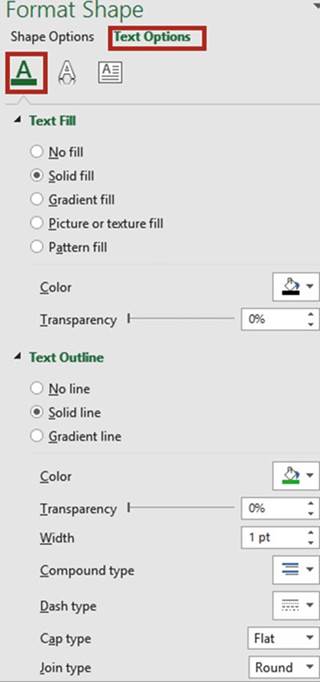
Figure 16-19. Text Options
dialog box
606
CHAPTER 16 ■ ENHANCING WORKBOOKS WITH MULTIMEDIA
15.
Click the Text Effects button. There are additional
effects here for Material and Lighting. See Figure 16-20. Go through each of the options for
these effects. You
will need to click each one. These options do not show the changes as you move your
mouse across them.
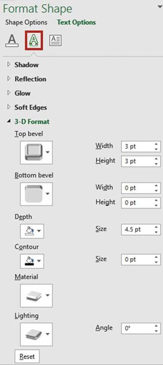
Figure 16-20. Text effects
WordArt can be transformed to follow paths
or to be warped in to real attention grabbers.
607
CHAPTER 16 ■ ENHANCING WORKBOOKS WITH MULTIMEDIA
In this exercise you will make text follow a path around a circle.
1.
Create a new worksheet.
2.
Click the Ribbon�s Insert tab. In
the Text group, click WordArt. Select the first letter A
in the
gallery.
3.
Change the text to say Professor
Office.
4.
In the Ribbon�s Size group, change
both the height and width to 3.94.
5.
Drag the border up so that it is near the top of your window. See Figure 16-21.
Figure16-21.Dragtheborderupasshownhere
6.
In the Ribbon�s WordArt Styles group, click Text Effects. Click Transform. Under Follow Path,
click the first shape
(Arch Up).
7.
Click the Ribbon�s Insert tab. In
the Text group, click WordArt. Select the first letter A
in the
gallery.
8.
Change the text to say Computer
Tutorials.
9.
In the Ribbon�s Size group, change
both the height and width to 3.94.
10.
In the Ribbon�s
WordArt Styles group, click Text Effects. Click Transform. Under Follow Path, click the second shape
(Arch Down).
11.
Drag the border up so that the text aligns underneath the Professor Office text as shown in
Figure 16-22.
12.
Click the Ribbon�s Insert tab. In the Illustrations group, click
Shapes and select the oval.
13.
Hold down the Shift key and drag it out so that it makes a
perfect circle within the text as shown in Figure 16-22.
This could be used for a logo. You could add more text within the circle.
You could jazz it up by applying
a 3-D or other effect to the circle.
608
CHAPTER 16 ■ ENHANCING WORKBOOKS WITH MULTIMEDIA

Figure16-22.Makeacirclewithinthetext
14.
Click the Ribbon�s View tab. In the Show group, uncheck Gridlines.
Adding and Modifying Shapes
Excel provides a large gallery
of eight groups of shapes.
See Figure 16-23. There is also a group that contains the shapes that you have used most recently. Shapes
are located
on the Ribbon�s Insert tab, in the
Illustrations group. To use a shape,
click where you want it, and then drag it out to the size you need.
Holding down the Shift key while you drag limits
the movement of some shapes;
for example, lines
will be kept straight, a rectangle shape
will be perfectly squared and an oval shape
will be a perfect circle.
You can add, alter, and delete shapes.
609
CHAPTER 16 ■ ENHANCING WORKBOOKS WITH MULTIMEDIA
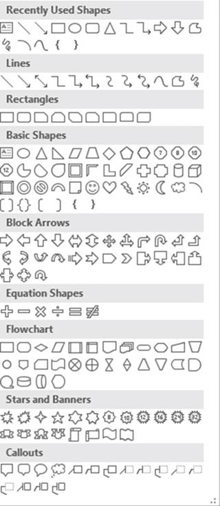
Figure16-23.Galleryofeightgroupsofshapes
For this practice we will use Shapes to create a portion of a flowchart. See Figure 16-24.
610
CHAPTER 16 ■ ENHANCING WORKBOOKS WITH MULTIMEDIA
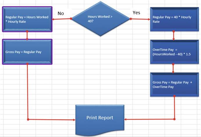
Figure16-24.Thiswillbeyourfinalresultfromthisexercise
1.
Create a new worksheet. Name the worksheet Shapes.
2.
Click the Ribbon�s Insert tab. In
the Illustrations group, click the
Shapes button.
3.
Select the Diamond shape in the Flowchart group. The cursor turns into a crosshair.
4.
Click the gridline
below row 12 and on the gridline
between columns F and G. Drag down and to the right.
Expand the shape until it almost takes four columns.
See Figure 16-25.
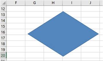
Figure16-25.Yourshapeshouldbethesamesizeandlocation
611
CHAPTER 16 ■ ENHANCING WORKBOOKS WITH MULTIMEDIA
5.
Click the Ribbon�s
Format tab. In the Shape Styles group,
click the More button for the Styles
gallery. In the last row of the Theme Styles
group, click the blue-colored style.
6.
Click the Ribbon�s
Insert tab. In the Illustrations group, click the Shapes button.
In the Flowchart group, click
the first shape.
It is a rectangle. Click
the left corner of where you want the rectangle
to start.
7.
Right-click the rectangle. Select Size and Properties. Enter
1 for Height and 2 for Width.
See Figure 16-26.
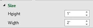
Figure16-26.Entertheheightandwidth
8.
Move the rectangle so that it aligns as shown in Figure 16-27.
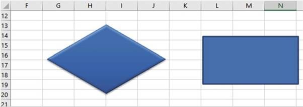
Figure16-27.Aligntherectanglewiththediamondasshownhere
9.
With the rectangle
selected click the Ribbon�s Format
tab. In the Styles group,
click the More button for the Styles
gallery. In the last row of the Theme Styles
group, click the blue-colored style.
10.
Press Ctrl + C to copy the rectangle. Press Ctrl + V four times to create four copies of the
rectangle.
11.
Drag the rectangles so they are positioned as shown in
Figure 16-28. Don�t
worry about exact placement; we will
align them next.
612
CHAPTER 16 ■ ENHANCING WORKBOOKS WITH MULTIMEDIA
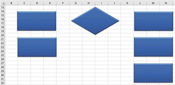
Figure 16-28.Drag
the rectangles so they are positioned as shown
12.
Hold down the Ctrl key and click the three rectangles on the right side.
13.
Click the Ribbon�s
Format tab. In the Arrange
group, click the Align button
and then select
Align left. The left border
of the three rectangles should
now be aligned.
14.
Click the Ribbon�s
Format tab. In the Arrange
group, click the Align button
and then select
Distribute Vertically. This makes the rectangles evenly
spaced apart vertically. Click a blank cell to deselect the three rectangles.
15.
Hold down the Ctrl key and click the two rectangles of the left side. Click
the Ribbon�s Format
tab. In the Arrange group,
click the Align
button and then select Align
left. The left border of the two rectangles should
now be aligned. Click a blank cell to deselect
the two rectangles.
16.
Hold down the Ctrl key and click the second
rectangle on the left and the second rectangle on the right.
Click the Ribbon�s
Format tab. In the Arrange
group, click the Align button and then select Align
bottom.
17.
Click the Ribbon�s
Insert tab. In the Illustrations group, click Shapes.
In the Flowchart group, click
the Document icon.
Place the cursor
where the top left corner
of the document shape is to start
and then drag it out so that it is in the same location
and size as shown in Figure 16-29.
613
CHAPTER 16 ■ ENHANCING WORKBOOKS WITH MULTIMEDIA
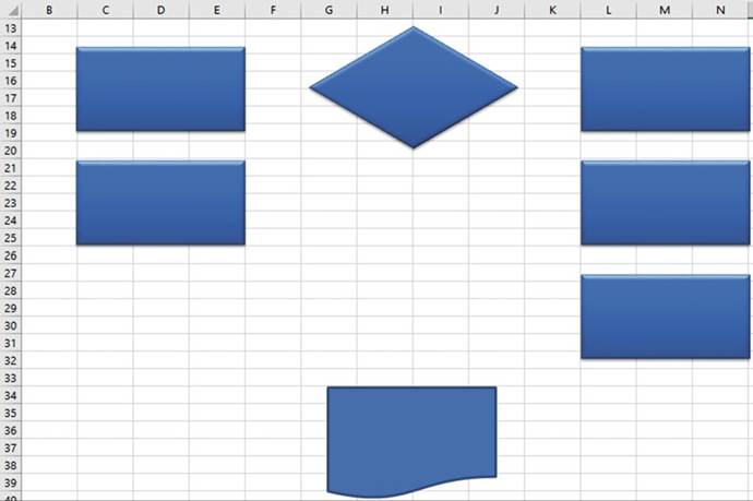
Figure 16-29.Drag
the Document icon out so that it is the same size and in the same location as shown here
18.
With the document shape selected, click the Ribbon�s Format tab. Click the More button for the
Styles gallery. In the Theme styles group, click the blue color in the last row.
19.
Now we can tie our shapes together
with arrows:
a.
Click the Ribbon�s Insert tab.
b.
In the Illustrations group, click shapes.
c.
In the lines group, click the second icon (the arrow).
d.
Hold down the Shift key and draw the arrow from the right
corner of the decision symbol to the rectangle to its right.
e.
Holding down the Shift key makes the arrow stay in a straight line.
20.
Next, let�s format the arrow:
a.
Click the arrow.
b.
Click the Ribbon�s Format tab. In
the Shape Style group, click Shape Outline.
c.
In the Standard Colors click red.
d.
In the Shape Style group, click
Shape Outline. Click Weight,
select 2 �.
e.
In the Shape Style group, click Shape Outline.
f.
Click Arrows, select the arrow with the circle on one end and the arrow on the other.
614
CHAPTER 16 ■ ENHANCING WORKBOOKS WITH MULTIMEDIA
21.
Right-click the arrow then select Set
as Default Line.
22.
Click the Ribbon�s
Insert tab. In the Illustrations group, click Shapes.
The first group in the Shapes is Recently
used Shapes. The arrow should be in this group.
Since you made changes to the look of the arrow and set it as the default line, the arrow line that you
select from here will look exactly like the arrow line you just created.
Select the arrow from the Recently used Shapes.
23.
Draw the arrow lines as shown in Figure 16-30. You can also speed up the process
of doing this without having
to go back to the menu every
time by copying
and pasting the arrow lines
and then moving
them where you want them.
You can rotate the lines
and resize them.
If they aren�t in the exact location
you want, you can use your keyboard
arrow keys to nudge them in to place.

Figure16-30.Drawthearrowlinesasshownhere
24.
Next we will draw the straight lines that connect the left
and right rectangles to the arrows pointing to the document icon:
a.
Click the Ribbon�s Insert tab. In
the Illustrations group, click
Shapes.
b.
In the Lines group, click the first line (the straight line).
615
CHAPTER 16 ■ ENHANCING WORKBOOKS WITH MULTIMEDIA
c.
Draw a line down from the second rectangle on the left and connect
it to the arrow line going to the document
icon. Since you created a default line that
has an arrow, we are going to have to remove the arrow.
d.
Right-click the line you just created and then select Format Shape.
e.
Click End Arrow type and then
select No Arrow. See Figure 16-31.
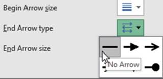
Figure 16-31. Select the No Arrow type
25.
Press Ctrl + C to copy the line. Press
Ctrl + V to paste it. Drag the pasted line so that it connects the bottom right rectangle to the line
connecting to the document
icon. Change the size to make it fit. Make any other necessary adjustments. Your flowchart should now look
like the one in Figure 16-32.
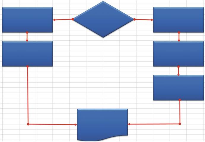
Figure16-32.Yourflowchartshouldnowlooksimilartothis
616
CHAPTER 16 ■ ENHANCING WORKBOOKS WITH MULTIMEDIA
26.
Now you can add the text:
a.
Click the top left rectangle.
b.
Enter the text Regular Pay = Hours
Worked * Hourly Rate
c.
Click the Ribbon�s Home tab. In the Alignment
group, click the Middle Align button.
d.
Enter and align the text in the same manner for the other
shapes. Enter the text as follows:
�
Second rectangle on left: Gross Pay = Regular Pay
�
Decision shape: Hours Worked >
40?
�
First rectangle on right: Regular
Pay = 40 * Hourly Rate
�
Second rectangle on right: OverTime Pay = (HoursWorked � 40) * 1.5
�
Third rectangle on right: Gross Pay = Regular Pay + OverTime Pay
�
Document shape: Print Report
e.
Increase the
size of the font in the Document Shape. Your
flowchart should look like the one in
Figure 16-33.
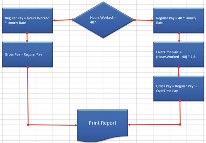
Figure16-33.Yourflowchartshouldnowlooksimilartothis
617
CHAPTER 16 ■ ENHANCING WORKBOOKS WITH MULTIMEDIA
27.
We will next add the text No to the left of the decision symbol and the text Yes to
its right:
a.
Click the Ribbon�s
Insert tab. In the Text group, click Text Box. The cursor
changes to a down arrow.
b.
Drag out a rectangle to the left of the decision symbol. Type No
in the text box.
c.
Right-click in the text box and then select Format Shape. Under Line select the option
No line. This removes
the text box border. Increase
the font size for the text to 16.
d.
Click the outside
border of the text box. Press
Ctrl + C to copy it. Press Ctrl + v to paste it. Move
the pasted text to the right of the decision
symbol.
e.
Change the text to Yes.
f.
Make any necessary movements.
Grouping
and Ungrouping Shapes
If you want to apply the same properties to multiple objects
you can make those objects
a group. If you move one object,
the entire group
moves. If you change a property of one object
Excel makes the same change to every
object in the group.
1.
Click the top right rectangle. Hold down the Ctrl key and click the other two right rectangles.
2.
Click the Ribbon�s
Format tab. In the Arrange
group, click the group button and then select Group.
3.
Click the top left rectangle. Hold
down the Ctrl key and click the other left rectangle.
4.
Click the Ribbon�s
Format tab. In the Arrange
group, click the group button and then select Group.
5.
Click the Ribbon�s
Format tab. In the Arrange
group, click the Selection pane button. The pane shows every object
with an eyeball to the right of it. See Figure 16-34. Clicking
an eyeball hides the object
associated with it. If you click an eyeball to the right of a group, it hides the entire group.
The hidden object
or group displays
a horizontal line. Clicking the horizontal line redisplays the object.
618
CHAPTER 16 ■ ENHANCING WORKBOOKS WITH MULTIMEDIA
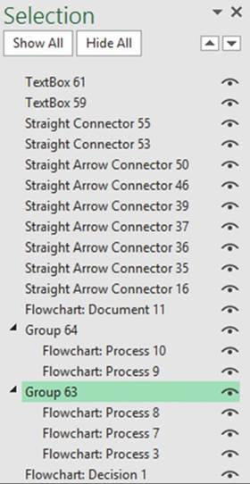
Figure16-34.Everyobjecthasaneyetotherightofit
6.
Double-click the group name for the right three rectangles. Change the name to RightRectangles.
7.
Click the eyeball
for the first right rectangle. Click the horizontal line to bring
it back. Click the eyeball for the RightRectangles group. Click the horizontal line to bring the group
back. Click on the word RightRectangles.
8.
Click the Ribbon�s Format tab. In the WordArt Styles group, click the Format Text Effects button
which launches the Format Text Effects task pane. See Figure 16-35.
619
CHAPTER 16 ■ ENHANCING WORKBOOKS WITH MULTIMEDIA
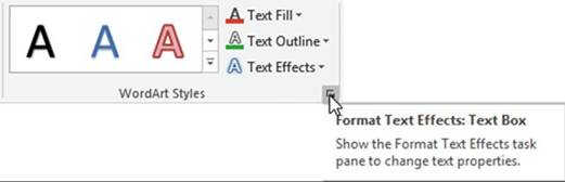
Figure16-35.Ribbon�sWordArtStylesgroup
9.
Click Lighting and select Sunset
under the Warm category. Click Top bevel and select
Round.
10.
In the Selection
pane, click the group for the two left rectangles. Change the name of the group to LeftRectangles. See
Figure 16-36.
Figure16-36.ChangethenameofthegrouptoLeftRectangles
620
CHAPTER 16 ■ ENHANCING WORKBOOKS WITH MULTIMEDIA
11.
In the Format Shape button
pane:
a.
Click Contour and select purple.
b.
Change the size to 5pt.
c.
Click Top Bevel then select Cutout.
d.
Change the width to 7 and the height to 5.
12.
Click the Ribbon�s
Format tab. In the Arrange
group, click the Group button
and then select
Ungroup. Click one of the rectangles on the right.
Click the Group button and then select
Ungroup.
13.
Close the Select pane.
14.
Click the Ribbon�s
Insert tab. In the Illustrations group, click Shapes.
Click the first shape in the Callout
group. Draw the callout to the upper left of the decision
shape.
The callout
has a yellow circle for one of its handles.
You can drag this circle toward the
object you want the Callout to be coming from.
15.
Drag the yellow circle toward the decision symbol. Type the text Cloud
Application
in the Callout shape. Align the text.
16.
You can change
any shape into another shape.
Let�s give the cloud application a cloud shape:
a.
In the Insert
Shapes group, click the Edit Shape button then select
Change Shape then select the Cloud Callout.
b.
Drag the yellow circle from the Cloud Callout to the decision shape.
621
CHAPTER 16 ■ ENHANCING WORKBOOKS WITH MULTIMEDIA
c.
Make any necessary changes to the size and shape of the
callout. See Figure 16-37.
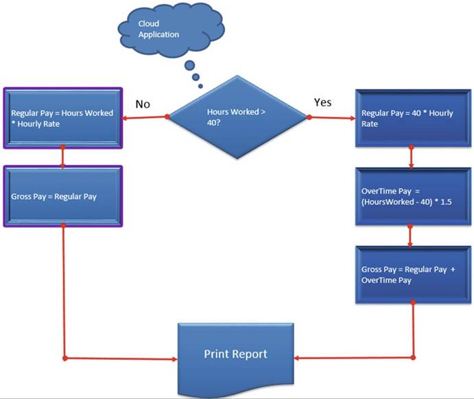
Figure 16-37. Create a Cloud shape
In this exercise you will practice changing the shape
of an object and moving one object in front of another.
1.
Create a new worksheet.
2.
Click the Ribbon�s Insert tab. In
the Illustrations group, click
Shapes.
3.
In the Basic Shapes group,
click the heart. Drag out the
heart in the middle of your window.
4.
In the Shape Styles group, click
Shape Fill and select the color red.
622
CHAPTER 16 ■ ENHANCING WORKBOOKS WITH MULTIMEDIA
5.
In the Insert Shapes group, click the Edit Shape button and then
select Edit Points.
6.
Two
small black handles have been added to the heart. Move your cursor over the top one and drag it up. Two
lines appear with a square at the end of each line. Practice moving the squares to change
the shape and size of the heart. See Figure 16-38.

Figure 16-38.Move
the squares to change the shape and size of the heart
7.
In the Illustrations group, click Shapes. In the
Stars and Banners group, click the third banner (curved-up ribbon).
8.
Drag out the banner below the heart.
9.
Move the heart
on top of the banner.
The banner moves
behind the heart
because the heart
was added first.
10.
In the Arrange
group, select Send Backward. The banner should
now be in front of the heart.
See Figure 16-39.

Figure16-39.Thebannershouldappearinfrontoftheheart
623
CHAPTER 16 ■ ENHANCING WORKBOOKS WITH MULTIMEDIA
In this exercise you will make an image take the shape of a circle.
1.
Create a new worksheet
2.
Click the Ribbon�s Insert tab. In
the Illustrations group, click the
Shapes button.
3.
In the Basic Shapes group, click the oval.
4.
Hold down the Shift key while you drag out the oval; this will make a
perfect circle.
5.
Click the Format tab. In the
Shape Styles group, click the Shape
Fill down arrow.
6.
Select Picture.
7.
Click Browse. Browse
to the image ShapeImage. Click the Insert button. The picture takes the shape of the circle. See Figure
16-40.

Figure16-40.Picturetakestheshapeofthecircle
In the last two sections, you have learned
how to create decorative text using WordArt,
which gives your text much more impact.
You have seen that Excel provides a large number of predefined shapes such as arrows, stars, banners,
callouts,
and so on, whose shape and color you can modify. Next, you will learn how to use SmartArt. SmartArt
takes shapes to another level by combining
multiple shapes with text to create various
customizable diagrams. There
are nine categories of diagrams and each one contains many layouts to choose from. You can also apply styles
to the layouts.
624
Using SmartArt
CHAPTER 16 ■ ENHANCING WORKBOOKS WITH MULTIMEDIA
SmartArt is a collection of customizable diagrams
that are categorized into groups such as Processes, Hierarchy, Matrixes, Pyramids, and so on. The All
category shows
all of the diagrams from the other categories. You access Choose
a SmartArt Graphic
dialog box and all the diagrams appear
via the SmartArt button in the Insert
tab�s Illustrations group.
See Figure 16-41.
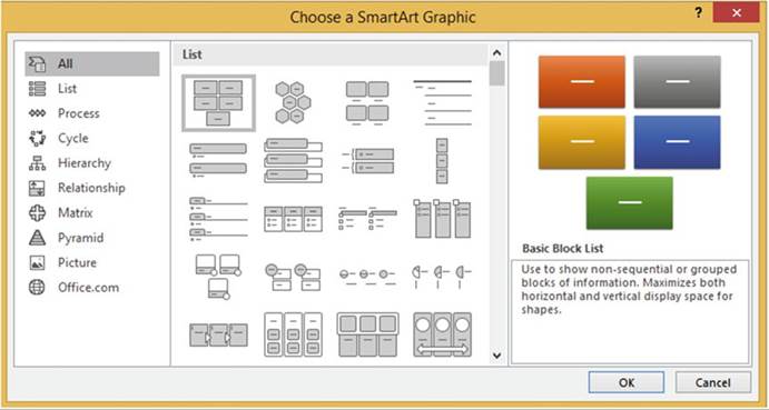
Figure 16-41.The
All category shows
all of the diagrams from the other
categories
It is best if you draw out how you want your
diagram to look before you start creating it in Excel. In this practice exercise you will create the
organizational
chart shown in Figure 16-42.
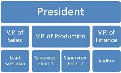
Figure16-42.Youwillcreatethisorganizationalchart
625
CHAPTER 16 ■ ENHANCING WORKBOOKS WITH MULTIMEDIA
1.
Create a new worksheet.
2.
Click the Ribbon�s Insert tab. In
the Illustrations group, click
SmartArt.
3.
Click each category in the left pane to view the different
diagrams. The All group displays all of the available diagrams.
4.
Click Hierarchy in the left pane. Click the Table Hierarchy in the right
pane. It is the last diagram in the second
row. Then click OK.
There is an arrow
button that appears
on the left side of the diagram.
See Figure 16-43. Clicking this button
turns the Text pane on and off. We will first change
the Text pane so
it matches the way we want the organizational chart
to look.
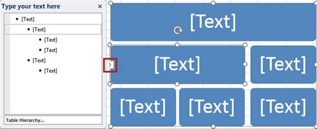
Figure16-43.ThearrowbuttonturnstheTextpaneonandoff
5.
Click the third text line in the Text pane. See Figure
16-44. Click the Ribbon�s Design
tab. In the Create Graphic
group, click the Promote button.
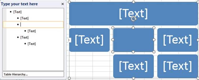
Figure16-44.Thetextblockfromthebottomrowismoveduptothesecondrow
626
CHAPTER 16 ■ ENHANCING WORKBOOKS WITH MULTIMEDIA
6.
In the Create Graphic group, click the Demote button. The
text block moves back down to the third row.
7.
Let�s perform the same function using a different method. Hold down the Shift key while pressing
the Tab key to promote the text block.
8.
Press the Tab key to demote the text block.
9.
Hold down the Shift key while pressing the Tab key to promote the text block back
again.
10.
We need to have two text blocks
below the second
row�s second text box. In the Create
Graphic group, click the Add Shape�s down arrow button.
Select Add Shape Below.
11.
Click the second Text block in the Text pane. In the Create Graphic
group, click the Add Shape�s
down arrow button.
Select Add Shape Below.
Now that we have the Text blocks in the order that we want we can enter the titles
for the positions.
12.
Enter the title for each position by entering the title either in the chart or in the Text pane.
Entering the title in either one will enter it in the other.
See Figure 16-45. After
typing V.P. of Sales press Enter then press the Tab key. to add the block below it.
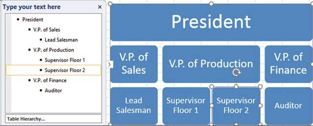
Figure 16-45.Enter
text in the pane and it will appear in the chart
and vice versa
13.
Click the Ribbon�s Design tab. In the Layouts group, click the Change Layout button.
14.
Click the third diagram in the first row. This is the Name and Title organizational chart. The
benefit
of this chart
is that besides
entering the title
for each position
you can enter the name of the person in that position. Just click in each text box and enter the names. See
Figure 16-46. Add your own names.
All the grid lines can be very distracting. There are two ways you can remove
the lines. One is
by turning off the grid lines. The other is by using
fill.
627
CHAPTER 16 ■ ENHANCING WORKBOOKS WITH MULTIMEDIA
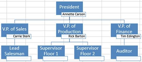
Figure16-46.NameandTitleorganizationalchart
Removing
the Gridlines by Turning Them Off
1.
Click the Ribbon�s
View tab.
2.
In the Show group, remove the check for Gridlines.
This removes the gridlines for the entire
worksheet. If you aren�t going to be entering other data in the worksheet
cells, this is the best method.
3.
In the Show group, check the
Gridlines to restore them for the next exercise.
Removing
the Gridlines by Using Fill
1.
Select all the cells around
the chart.
2.
Click the Ribbon�s
Home tab.
3.
In the Font group, click the
Fill Color button and then select White.
4.
Click the down arrow for the border and select Thick Outside Border. See Figure
16-47.
628
CHAPTER 16 ■ ENHANCING WORKBOOKS WITH MULTIMEDIA
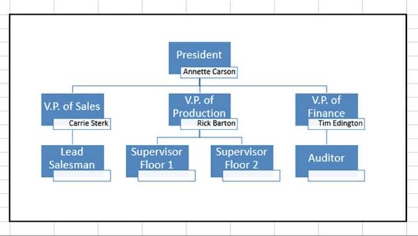
Figure
16-47.NameandTitleorganizationalchartwiththickoutsideborder
Now that we have the organizational chart the
way we want we can select one of many different layout choices.
5.
Click anywhere on the organizational chart.
6.
Click the Ribbon�s
Design tab. In the Layouts
group, click the second diagram
in the first row. This is the Picture Organization Chart.
7.
Click the picture icon
 �for the President.
This brings up the Insert Pictures window
where you can select a picture from your computer or from the Internet.
8.
Click Browse. The
Insert Picture window displays. Browse
to the picture President. Click the
Insert button.
9.
Follow the same process for the V.P. of Sales. Use
the
Image VPofSales. See Figure 16-48.
629
CHAPTER 16 ■ ENHANCING WORKBOOKS WITH MULTIMEDIA
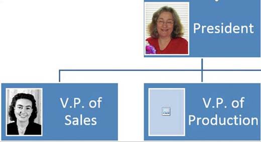
Figure16-48.UsetheimageVPofSales
10.
Click inside a blank area directly to the left or right
of the president shape to select the entire organizational chart. Click the Ribbon�s
Design tab.
11.
Click the More button for Layouts. Select
the Horizontal Hierarchy Chart.
12.
Click the Ribbon�s
Design tab. In the SmartArt
Styles group, click the Change
Colors button. Move your cursor
over the gallery
objects to see how they affect your chart.
13.
Select the first object under Primary Theme colors.
14.
Right-click the President shape in your chart. Select Change Shape.
15.
In the Stars and Banners group select Horizontal Scroll.
16.
Click the Ribbon�s
Format tab. In the Shape Styles group,
click Shape Fill. Click whatever
color you like. See Figure
16-49.
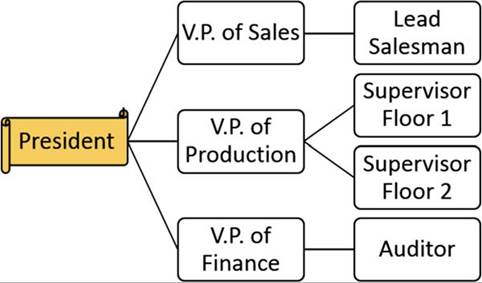
Figure16-49.SelectacolorforShapeFill
630
CHAPTER 16 ■ ENHANCING WORKBOOKS WITH MULTIMEDIA
You have learned how to create
impressive worksheets by using images,
shapes, and layouts.
Next you will learn
how to add audio and video that you or someone else has created
to a worksheet.
Inserting Sound
into a Worksheet
It is a very simple process to create your own audio sounds. You can buy a good inexpensive microphone and if
you have a laptop
it probably has a built-in
microphone. You can add audio to your workbook to provide instruction or to provide information about the
data in the workbook or an explanation of why things were done the way they were.
You can either embed the audio file into your workbook or create a link to the audio file. The same is true
for video files. If you create a link to the audio file, the file doesn�t
exist as a part of your workbook.
When you play the audio file Excel searches
for the file in the location (path) that you gave it. If you ever move your
file from that location, Excel will not be able to find it.
Add sound to your
worksheet by doing the following:
1.
Select the cell near which you want the sound inserted.
2.
Make sure the Insert
tab of the Ribbon is displayed.
3.
Click the Object tool in the Text group. Excel displays
the Object dialog box.
4.
Click the Create
from File tab.
5.
Use the controls on the dialog
box to locate a sound
file that you want included
with your document.
6.
Click OK. An icon that looks
like a speaker is inserted
in your document.
You can later listen
to your sound
file by simply
double-clicking the speaker
icon. You can also move the
icon to some other place on your worksheet
In this exercise you will embed an audio file into your worksheet.
1.
Add a new worksheet to your workbook.
2.
Click the Ribbon�s
Insert tab. In the Text group, click
the Object button.
The Object dialog
box displays.
3.
Click the Create from File tab.
See Figure 16-50.
631
CHAPTER 16 ■ ENHANCING WORKBOOKS WITH MULTIMEDIA
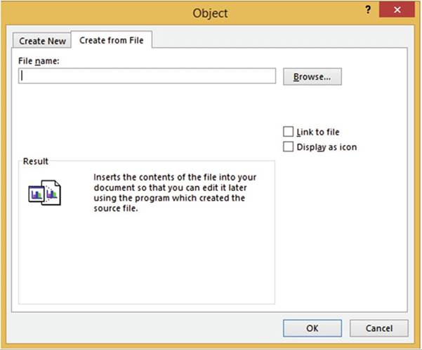
Figure16-50.CreatefromFiletabontheObjectdialogbox
4.
Click the Browse button and then find the file ExcelAudioFile.
5.
Click the OK button. Since
you didn�t select Link to file, the
file will be embedded into your workbook.
6.
Double-click the Audio icon. See Figure 16-51.

Figure16-51.Double-clickthisiconifyouwanttoplaytheaudiofile
The Open Package Contents dialog
box opens. See Figure 16-52.
632
CHAPTER 16 ■ ENHANCING WORKBOOKS WITH MULTIMEDIA
Figure16-52.OpenPackageContentsdialogbox
7.
Click the Open button. The
audio should start playing.
Inserting Video
into a Worksheet.
In order to play a video file in Excel
you will need to have a software
program that plays
video, such as Windows Media
Player.
Just like audio files, video files can be either embedded
into your worksheet
or linked to it. As mentioned previously, the problem with linking a file is that if you move that file
after you have created
the link or distribute it to others,
Excel will not be able to find it. If you do not choose to link the file, the file will become a part of
your workbook. If the video file is large your workbook of course will take up more space.
Video and Audio files
are added the same way to a worksheet.
In this exercise you will embed a video file into your worksheet.
1.
Place your cursor where you want the icon for the video file to be.
2.
Click the Ribbon�s
Insert tab. In the Text group, click
the Object button.
The Object dialog
box displays.
3.
Click the Create from File tab.
4.
Click the Browse button and then find the file Transpose. Click the
OK button.
5.
Double-click the Video icon. See Figure 16-53.
633
CHAPTER 16 ■ ENHANCING WORKBOOKS WITH MULTIMEDIA

Figure16-53.Double-clicktheVideoicontostartthevideo
6.
The Open Package Contents
dialog box opens. Click the Open button.
The video file starts playing
in your computer�s default video player.
Using Bing Maps
Using Excel�s Bing Maps you can create
a visual representation of your data in any location in the world.
The first column of the data must be an address,
city, state, country,
zip, latitude/longitude, or a combination.
Any columns following that must be numeric data.
The problem with using a city is that there
may be many cities with the same name. You can concatenate a city with a state
or country name.
In this exercise you will create maps that reflect the revenue created in
different cities.
1.
Open the Chapter 16 workbook. Select
the worksheet named Maps.
The examples in this worksheet
use Revenue for the numeric
amount. The values
could be anything
(e.g., city or state populations, growth rates, death
rates, number of employees in a company
working in that location, etc.).
2.
Click the Ribbon�s
Insert tab. In the Add-ins
group, click the Bing Maps button. The Bing Map displays. See Figure 16-54.
634
CHAPTER 16 ■ ENHANCING WORKBOOKS WITH MULTIMEDIA
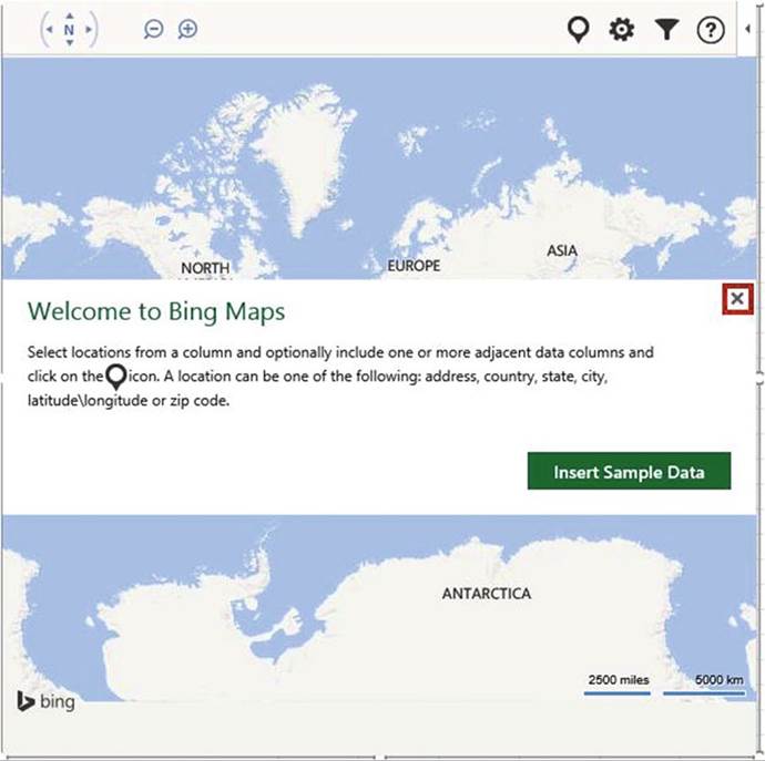
Figure 16-54. Bing Maps

3.
Click the X to close the opening message.
4.
Select the cell range A1:B4. Click the Show Location button�� in the upper right corner.
Bing displays
a map with a circle in each of the three states.
See Figure 16-55. The circle represents the amount of the numeric
data. Illinois had the largest
amount so its circle is the largest.
635
CHAPTER 16 ■ ENHANCING WORKBOOKS WITH MULTIMEDIA

Figure16-55.Circlesrepresenttheamountofrevenueforthatlocation
Select the cell range A6:C11.
Click the Show Location button
 . The map displays with a circle at each of our locations. See Figure 16-56. Since we provided
two numeric columns
it displayed the first column�s
value as the outer circle and the second column�s
value as the inner circle.
The map displays a legend to show which value goes with which color.
. The map displays with a circle at each of our locations. See Figure 16-56. Since we provided
two numeric columns
it displayed the first column�s
value as the outer circle and the second column�s
value as the inner circle.
The map displays a legend to show which value goes with which color.
636
CHAPTER 16 ■ ENHANCING WORKBOOKS WITH MULTIMEDIA
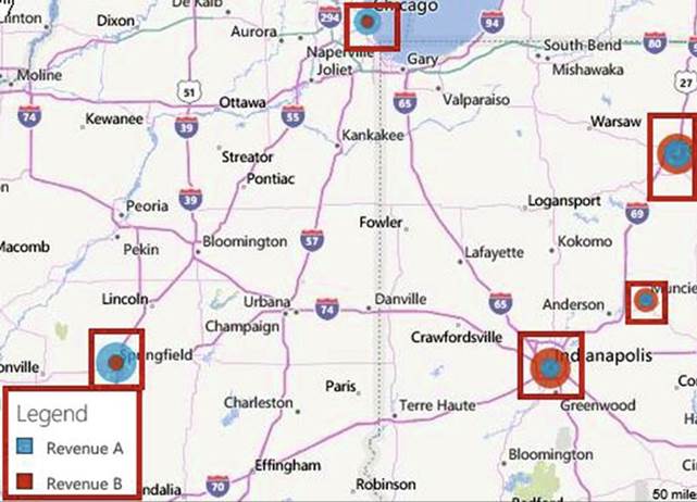
Figure 16-56.Legend
identifies the colors
for the different revenue columns
The circles are okay when viewing two numeric
values, but when using more than two columns it is really difficult to
identify the colors. Instead of
using circles you can use a pie
chart.
5.
Select the cell range A13:D17. Click the Show Location button
 .
.
6.
Click the Settings
button
 . Select Pie Chart under
Multiple Data Point Display. See Figure 16-57. Excel
lets you select
a different color
for each of the three
pie slices.
. Select Pie Chart under
Multiple Data Point Display. See Figure 16-57. Excel
lets you select
a different color
for each of the three
pie slices.
7.
Pick whatever colors you want. When you have finished picking your colors, click the arrow within
the circle to
return to the map.
637
CHAPTER 16 ■ ENHANCING WORKBOOKS WITH MULTIMEDIA
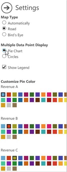
Figure 16-57. Select Pie Chart
The pie charts should display using the colors you selected. See Figure 16-58.
638
CHAPTER 16 ■ ENHANCING WORKBOOKS WITH MULTIMEDIA

Figure16-58.Valuesarerepresentedbypiecharts
Excel provides three buttons at the top left of the map. The first button lets you pan the map. The second
and third buttons let you zoom in and out. See Figure 16-59.

Figure16-59.Buttonsforpanningandzoominginandout
8.
Try dragging your mouse cursor
around inside the circle of the pan button. When your mouse is on the map the cursor
shows as a hand. You can get the same results as using the pan tool by dragging
the hand cursor
on the map.
9.
Moving your cursor
over the Zoom in or Zoom out button displays
the drag bar as shown in Figure
16-60. You can drag the bar across
the lines to zoom. You can also just click the Zoom in and Zoom out buttons. Try using both methods.

Figure 16-60. Zoom drag bar
10.
Select the cell range A19:B22.
Click the Show Location button
 . Because all of the locations are in the same city, the map is zoomed in.
639
CHAPTER 16 ■ ENHANCING WORKBOOKS WITH MULTIMEDIA
11.
Click the Settings button
 . Under Map Type, Select Bird�s Eye. Click the arrow within the circle to return to the map. Zoom
in to the street
level. See Figure 16-61. The locations don�t
have to be of the same type. You can have a mix of cities, states, countries, zip codes, address, and so on,
as shown in Table 16-1.
. Under Map Type, Select Bird�s Eye. Click the arrow within the circle to return to the map. Zoom
in to the street
level. See Figure 16-61. The locations don�t
have to be of the same type. You can have a mix of cities, states, countries, zip codes, address, and so on,
as shown in Table 16-1.

Figure 16-61. Street-level map
Table16-1.LocationsofMixedTypes
|
Location
|
Revenue
|
|
Kentucky
|
7500
|
|
Chicago
|
4500
|
|
France
|
5000
|
|
Germany
|
8000
|
|
46341
|
7000
|
|
550 N. Clinton St.,
Fort Wayne
|
6000
|
Moving,
Resizing, and Deleting the Map
You can move the map by placing
your cursor on the border above the buttons shown in Figure 16-62. The cursor changes to four arrows.
You can then drag the map to wherever you want.
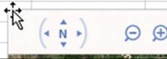
Figure 16-62.When your cursor changes to four arrows
you can drag the map
640
CHAPTER 16 ■ ENHANCING WORKBOOKS WITH MULTIMEDIA
If you click while on the border
the sizing handles
display. See Figure
16-63. When you move your cursor over a sizing
handle it changes
to a double arrow. You can drag toward the map to decrease its size or drag away from the map to increase
its size.
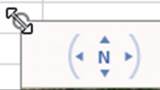
Figure16-63.Whenthecursorisadoublearrowyoucanresizethemap
You can delete
the map when the sizing
handles are displayed by pressing the delete key.
Summary
You have seen how multimedia can have a visual impact
as well as improving how quickly the user can grasp what you want him or her to know. Multimedia makes your
worksheets look more polished
and professional as well as giving you much more power to convey your message.
You can add pictures
to your worksheet from either your computer or the Internet. You have seen how
you can even create a logo with WordArt by making the text follow
a path
Screenshots can be used to capture
an entire screen
or a selected portion from a web site or other application and then place
that capture in the current
worksheet. The capture
is added to your worksheet as an Image.
You can alter it in the same way you can alter any other image.
You have learned how to use Shapes and SmartArt to create flowcharts, organizational charts, and other
types of layouts. You can add, alter,
and delete a wide variety
of shapes.
It is very simple
to add audio and video.
You can either
embed the files
into your workbook
or link to them.
You can buy a good inexpensive microphone to record your audio notes.
In order to play a video file in Excel,
you will need to have a software
program that plays
video, such as Windows media
player.
Bing Maps represent your spreadsheet data on a map. The map can be a city, state, country, or the world.
In the next chapter,
you will see how you can use macros to automate tasks
that you repeat
over and over again. Macros are a recording of a task. Once you have this recording saved, you can run it as
many times as you need to.
641
CHAPTER
17
Automating Task with Macros
Macros can be big timesavers for those tasks
you find yourself
performing over and over again.
Macros
enable you to record
a series of steps that you normally
use to perform a task,
store those steps,
and then automatically rerun those steps
whenever you want.
Macros can be quickly activated by assigning shortcut keys to them. If you think
you might forget
a macro�s associated shortcut key, then you can store it in the Quick Access Toolbar. You can also attach
macros
to buttons and other objects.
After
reading and working
through this chapter
you should be able to
�
Create a macro
that uses an absolute cell reference
�
Create a macro
that uses a Relative cell reference
�
Assign a macro to a button
�
Assign a macro
to the Quick Access Toolbar
�
Assign a macro to a shape
�
Create and update the personal workbook
�
Save a macro-enabled workbook
�
Use the VBA (Visual Basics
for Applications) Development Environment
�
Edit a macro
Creating (Recording) a Macro
Simple macros can be
created using the Macro Recorder. More complex macros can be created in the
Macro Editor. The Macro Recorder
records every keystroke and every mouse click from the time you start the recorder to the time you stop it.
Since it records everything that you do, don�t click any other cells or perform any steps other than those
that are
directly related to the task you want to perform.
The
Macro Recorder can be started
from three different locations:
�
On the View tab, in the Macros group, click the down arrow for the Macros button and select Start
Recording.
�
On the Developer tab, in the Code group,
click Record Macro.
�
On the Status
bar, click the Macro Start
Recording button

643
CHAPTER 17 ■ AUTOMATING TASK WITH MACROS
When you start
the recorder, a Record Macro dialog box opens where you will need to enter the
name you are assigning to the
macro, a shortcut key, and where you want the macro stored; you can also
provide a description of the macro so
that later you can remember what its purpose is. See Figure 17-1.
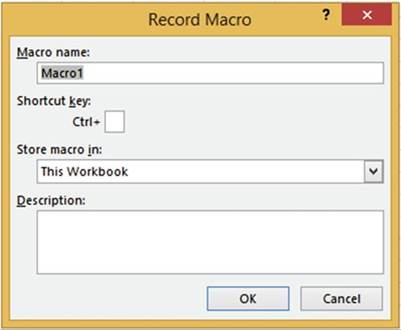
Figure17-1.Entriestomakebeforerecordingthemacro
There
are three places
you can store
your macro:
�
The current workbook
�
A new workbook
�
The Personal Macro Workbook
If you want to make the macros available for use in other workbooks, select Personal Macro Workbook. The
Personal Macro Workbook doesn�t exist until you save a macro to it. Excel saves the file as PERSONAL. xlsb.
This workbook is hidden and is opened automatically whenever you start Excel.
The macro we will create will apply
formatting to a cell. We will use
the Start Recording button on the status bar.
Recording the Macro
1.
Create a new workbook:
a.
Click the File tab and then select Save
As.
b.
Select the location where you want your workbook stored.
c.
Enter Macro_Practice
for the File name.
d.
Select Excel Workbook for the Save As type.
e.
Click the Save button.
644
CHAPTER 17 ■ AUTOMATING TASK WITH MACROS
2.
Look on your status bar and see if you have the Macro Start Recording button
 . If you don�t, then right-click the status bar, select the option for Macro Recording, and
then press the (Esc)ape key to hide the option window.
. If you don�t, then right-click the status bar, select the option for Macro Recording, and
then press the (Esc)ape key to hide the option window.
3.
Click inside cell A1.
4.
Click the Macro Recording button on the status bar. The Record Macro dialog box opens.
5.
The macro name can�t contain any spaces.
Type FormatEntry for the
Macro name.
The Shortcut key is currently
showing Ctrl + and a text box where you are to enter a keystroke
that will be used in addition to the Ctrl key. If you enter a lowercase
letter Excel requires
you to enter the Ctrl key
+ the letter that you entered for
the shortcut key. Unfortunately, just about all the shortcuts that use a Ctrl key and a lowercase letter
are already being used by Excel, so we will only be using uppercase
letters. If you enter an uppercase letter,
Excel adds a Shift key to the
shortcut; therefore you would need to enter
Ctrl + Shift + the letter you entered for the shortcut
6.
Click inside the text box and type Shift + F.
7.
Click the drop-down arrow for the Store Macro in drop-down box and select This Workbook
because we
only want to use the macro in the current workbook.
8.
For Description, type This is my first
macro. It will bold, italicize, change the font size to 16, and change the background color
to red.
9.
Click the OK button.
Every keystroke and mouse
click that
you make
from now
until you
click the
Stop
Recording button is
recorded, so don�t
click any
other cells
or any
command
buttons other than
what you
are instructed here to
do. You will
know when
you are recording a
macro because
the Macro
Start Recording button changes
to the
Macro
Stop Recording button
 . Look at
your status
bar; the
Macro Stop
Recording
button should be
displayed
. Look at
your status
bar; the
Macro Stop
Recording
button should be
displayed
10.
On the Ribbon�s Home tab, in the Font group, click the Bold and
Italics buttons. Change the font size to 16. Change the Fill Color to Orange, Accent 2, Lighter 80%. See
Figure 17-2.
645
CHAPTER 17 ■ AUTOMATING TASK WITH MACROS
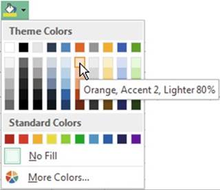
Figure17-2.ChangetheFillColortoOrange,Accent2,Lighter80%
11.
Click the Macro Stop Recording button
 �on the status bar.
Playing
Back the Macro
1.
Click cell C2.
2.
Type Hello.
3.
Press Ctrl + Enter.
4.
Press the shortcut keys you created for this macro Ctrl + Shift + F
All the keystrokes you used during the recording are now played back and
the text in C2 is formatted as
defined in the macro.
The Problem with Absolute Cell
References
When you record macros you can record them using absolute cell references, which is the default, or
you
can choose to record them using relative
cell references. When you record a macro using absolute
cell
references,
Excel records the exact location where you entered your data. None of your
pointer movements are recorded (such as using the up and down arrow
keys). Unfortunately, if you use Excel�s default absolute cell
references when using multiple cells, you may not get the results you expected.
This exercise will show the problem with absolute cell references so that
you will be able to identify it.
1.
Create a new worksheet. Change the name of the worksheet to �Absolute.�
2.
Click the Macro Start Recording button
 �on the status bar.
646
CHAPTER 17 ■ AUTOMATING TASK WITH MACROS
3.
Enter AbsoluteReference for the Macro name. (There
can be no spaces in a Macro name.)
4.
Enter Shift + A for the shortcut key.
5.
Store the macro in This Workbook.
6.
For the Description type Enter values into multiple cells using Absolute
Cell Referencing.
7.
Press the OK button.
8.
Click inside cell B4. Type the word Excel.
Press the tab key and then type 2016.
Press the tab key twice
and then type Macro.
Press the tab key twice
and then type Tutorial. Press Ctrl + Enter.
9.
Click the Macro Stop Recording button
.

10.
Click inside cell C6. On the View tab, in the Macros group, the
Macros button has
two parts.
Clicking the top half of the button
displays the Macro dialog box which displays
all of your macros. Clicking
the down arrow
on the bottom half of the Macros
button brings up a menu from which
you can select
View Macros. See Figure 17-3. This option also brings up the Macro dialog box.
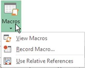
Figure17-3.ClickingthebottomhalfofMacrosbuttonbringsupamenu
11.
Click the down arrow for the Macros button and then select View Macros.
12.
The Macro dialog
box opens
showing all of the available
macros. Select the AbsoluteReference
macro.
Click the Run button. This is another way of
running a macro. You could have also used the shortcut you created, which was Ctrl + Shift + A. See
Figure 17-4.
647
CHAPTER 17 ■ AUTOMATING TASK WITH MACROS
The results are probably that cell G4 became the active cell.
This is because
it repeated the entries that you previously made rather than placing the entries starting
at cell C6. This is because Excel
uses absolute referencing by default, which doesn�t adjust
for any changes
in the row or columns.
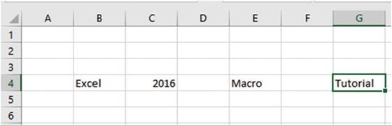
Figure17-4.ResultsofrunningtheAbsoluteReferencemacro
Absolute referencing is fine when you first apply formatting to a cell and
then apply that formatting to another cell,
as we did previously, but it
doesn�t work well for multiple entries.
You have
learned to create macros using Excel�s default absolute cell reference. In
Exercise 17-10 you will look at the code that Excel created for this
macro and how you can alter it.
Saving a Macro-Enabled Workbook
Workbooks that contain macros must be saved using a different file format than those used for other
workbooks. Workbooks that do not contain macros are usually saved with the extension .xlsx. Macro- enabled
workbooks need to be stored with the extension .xlsm.
We originally saved our Macro_Practice workbook as an Excel Workbook, but we have added macros
to the workbook since we did the save. If we try to save it again as an Excel Workbook
we will get a warning
message stating that if we continue with this save we will lose all the macros saved to this workbook.
1.
Click the Save button
 �on the Quick
Access Toolbar. See Figure 17-5.
�on the Quick
Access Toolbar. See Figure 17-5.
648
CHAPTER 17 ■ AUTOMATING TASK WITH MACROS
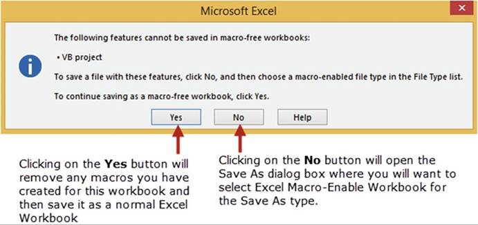
Figure 17-5.Warning message that is displayed if you try to save a workbook
as a normal workbook instead
of a macro-enabled workbook
2.
Click the No button.
3.
Click the down arrow for Save as type and then select Excel
Macro-Enabled Workbook. See Figure 17-6.
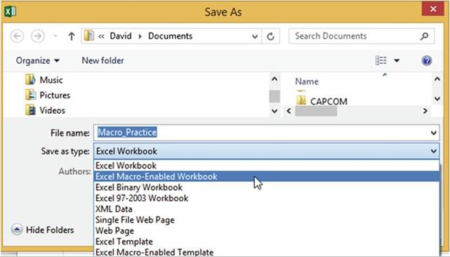
Figure17-6.SelectExcelMacro-EnabledWorkbook
649
CHAPTER 17 ■ AUTOMATING TASK WITH MACROS
4.
Click the Save button.
The workbook is saved as macro-enabled and the extension .xlsm is added to the file name. The
macros saved to the workbook will be available to use in the future.
Creating a Macro Using Relative Cell References
If you are creating a macro where you will be entering data into more than one cell you should use
relativecell references. As you have seen, absolute cell referencing for multiple cell entries
is relatively useless. It
doesn�t seem to make any sense why Microsoft decided not to make relative cell referencing the default.
We will create a macro the same way we did
for the AbsoluteReferencing macro
except that this time we will create it using the relative reference method.
1.
Close all open Excel workbooks. Create
a new Excel workbook.
2.
Click the View tab
on the
Ribbon. In the Window group
notice that there is a Hide and
Unhide button. Unless you
have previously
saved macros
to the
Personal Macro Workbook the Unhide
button should be currently unavailable.
3.
Click the down arrow of the Macros button and select Use Relative References.
4.
Click inside cell B4. Click the
Record Macro button on the Status bar.
5.
In the Macro dialog box, complete the following steps:
a.
Enter RelativeReferencing for
the name.
b.
Enter a capital R for the shortcut key.
c.
Change the storage location of the macro to Personal Macro Workbook.
d.
For the Description type Enter values into multiple cells
using Relative Cell Referencing.
e.
Click the OK button.
6.
Type the word Excel in cell B4. Press the tab key then type 2016. Press the tab key
twice and then type Macro. Press the tab key twice and then type Tutorial. Press Ctrl + Enter.
7.
Click the Macro Stop Recording button on the status bar.
8.
Click in cell C6. Click
the top half of the Macros button. You
should see the macro you created. Excel
has changed the name of the macro to reflect that it is being stored in the PERSONAL.XLSB file.
9.
Select the name of your new macro and then click the Run
button. This time all of the data displays in the new row.
10.
Click the View tab. In the Window
group the Unhide
button should now be available for use. Click
it. See Figure
17-7.
650
CHAPTER 17 ■ AUTOMATING TASK WITH MACROS
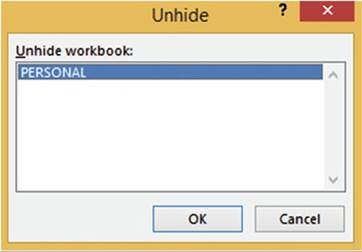
Figure 17-7. Unhide dialog box
11.
With PERSONAL workbook
selected click the OK button.
You should now be
looking at the PERSONAL workbook. It looks like a normal workbook with one worksheet. Its purpose is just to
make its macros available to other workbooks. On the Ribbon on the View tab in the Windows group click the
Hide button.
The PERSONAL workbook
should now be hidden and you should
be looking again at your original workbook.
12.
On the Ribbon, click the File
tab, click Save As.
13.
Select where you want the file to be saved.
Because the
workbook contains a macro it must be saved as macro-enabled.
14.
Change the Save as type to Excel Macro-Enabled Workbook. Name the workbook
Relative. Click the Save button.
15.
Click the
 �in the upper right corner to exit from Excel.
If you didn�t
save the Personal
Macro Workbook you will be asked to save the changes you made to it. See Figure 17-8. Click
Save.
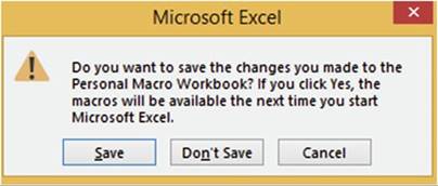
Figure 17-8.Excel
asks if you want to save the changes to the Personal
Macro Workbook
651
CHAPTER 17 ■ AUTOMATING TASK WITH MACROS
■
Note� I know the message says to click
Yes, but there
isn�t a Yes button. Click
the Save button.
Now whenever you start another
workbook the PERSONAL
workbook will be automatically loaded
but it will be hidden.
If you click the Unhide
button from now on you will see the PERSONAL
workbook.
Adding Macros to the Quick Access
Toolbar and Other Objects
So far we have seen that you can run a macro by typing its shortcut keys and seen how you can run it from the
Macros button. For easy and quick availability, you can add a macro
to the Quick Access Toolbar
or you can attach
it to a button or other object.
We will assign the RelativeReferencing macro you just created to the Quick Access Toolbar.
1.
Create a new Workbook.
2.
Right-click the Quick Access Toolbar. Select Customize Quick Access Toolbar. See Figure
17-9.
652
CHAPTER 17 ■ AUTOMATING TASK WITH MACROS
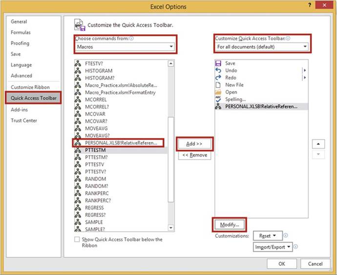
Figure 17-9. Excel Options dialog box
3.
From the left pane select Quick Access Toolbar.
4.
Under the Choose commands from drop-down
menu, choose Macros.
5.
Select PERSONAL.XLSB!RelativeReferencing.
Click the Add button.
■
Note� Because we saved
the macro RelativeReferencing to the Personal
Workbook, it is available to be used in all of our Excel workbooks.
5.
Under the Customize Quick Access Toolbar drop-down menu, choose For all documents
(default). The other choice for the
drop-down menu is to place the macro in the Quick Access Toolbar only when the current workbook
is being used.
6.
Click the Modify button. This brings up the Modify Button dialog box. See Figure 17-10.
653
CHAPTER 17 ■ AUTOMATING TASK WITH MACROS
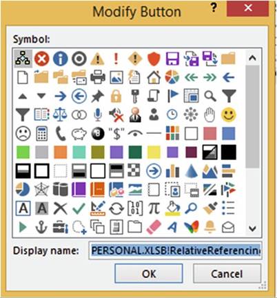
Figure 17-10. Modify Button dialog box
7.
Select whatever button
you want to associate with the macro.
The button that you select
will be placed
on the Quick Access Toolbar.
Click the OK button on the Modify
Button dialog box.
8.
Click the OK button in the Excel Options dialog box.
9.
Click cell A11. Click the button you
just created on the Quick Access Toolbar. The RelativeReferencing macro runs.
So far we have seen that you can run a macro from the Macros button or by typing its shortcut
keys. You have also learned how to get quick access to a macro by adding it to the Quick Access Toolbar. In
the next exercise, you will assign a macro to a shape that you can click to start the macro.
In this exercise, you assign a macro to a shape.
1.
Create a new worksheet.
2.
On the Ribbon click the Insert tab. In
the Illustrations group, click the
Shapes button.
3.
In the Flowchart group click the Flowchart:
Punched Tape icon. See Figure 17-11.
654
CHAPTER 17 ■ AUTOMATING TASK WITH MACROS
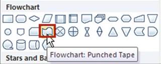
Figure17-11.SelecttheFlowchart:PunchedTapeicon
4.
Drag out the shape starting
in cell G2.
5.
On the Ribbon
click the Home tab. In the
Alignment group click the middle align button and the center
button. See Figure 17-12.
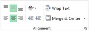
Figure 17-12. Ribbon�s Alignment
group
6.
Type Relative
Reference on the shape. Drag across the text to select it. Bold the text and increase its size until
it looks similar to the one in Figure 17-13. Click an empty cell to deselect
it.

Figure17-13.Makeyourbannerlooklikethis
7.
Right-click in the
center of the shape. Select Assign Macro. Select PERSONAL.
XLSB!RelativeReferencing and then click
the OK
button.
8.
Click an empty cell to deselect the shape.
9.
Click the cell where you want to start the macro and then click the shape.
655
CHAPTER 17 ■ AUTOMATING TASK WITH MACROS
The Macros button is on the Ribbon�s View tab. This means you have to click the View tab when you want to
view the macros or if you need to specify if you want Absolute Cell Referencing or Relative
Addressing. To make these features available no matter what the active Ribbon tab is, we will add the Macro
button to the Quick Access Toolbar in the next exercise.
We will place the Macros button on the
toolbar so that you will not need to go to the
View tab every time you want to run or edit a macro.
1.
Click the File tab on the Ribbon. Click
Options.
2.
From the left pane select Quick Access Toolbar.
3.
Under the Choose commands
from drop-down menu, choose Popular commands.
4.
Scroll to the bottom of the list and find
View Macros. Select View Macros. Click the
Add button.
5.
Click the OK button.
6.
Click the View Macros button on the Quick Access
Toolbar. Click the Cancel button.
Adding
the Developer Tab to the Ribbon
If you are creating VBA code or assigning a macro to a button
you will need to do this in the Visual Basic Environment which can only be accessed
through the Ribbon�s
Developer tab. If you don�t see a Developer tab on your Ribbon you will need to add it by performing the
following steps:
1.
Click the File tab
on the Ribbon. Select Options in the left pane to open the Excel Options
dialog box.
2.
Click Customize
Ribbon in the left pane. Select Developer in the right pane. Click
the OK button. See Figure 17-14.
656
CHAPTER 17 ■ AUTOMATING TASK WITH MACROS
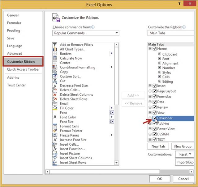
Figure 17-14. Select Developer
You should now see a Developer tab on
the Ribbon.
We will assign the same macro to a button.
1.
Create a new worksheet.
2.
On the Ribbon, click
the Developer
tab.
In the Controls Group click
the Insert
Button. Excel has two types
of controls: Form
Controls and ActiveX Controls. Both
types have
some of
the same
controls. You
cannot assign macros to ActiveX Controls, as
you can
with Form
controls. See Figure 17-15.
657
CHAPTER 17 ■ AUTOMATING TASK WITH MACROS
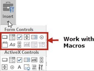
Figure 17-15. Form Controls
3.
Select the first form control, which is the button. Move
the cursor down into the spreadsheet
area. The cursor will change to a
crosshair.
4.
Starting in cell C2 drag down and to the right until you
have created enough area for a button.
5.
The Assign Macro dialog box appears. Click
PERSONAL.XLSB!RelativeReferencing. Click the OK button.
6.
Right-click the button and select Edit Text. Change the
text on the button from Button 1 to Practice.
7.
Click inside any empty cell to deselect the button. Click the button you just created.
Sharing the Personal Workbook with Others
You can use the Personal Workbook
(Personal.xlsb) on other computers or share it with others by
e-mailing them the file or copying
it to an external drive and then they could copy the file into the XLSTART folder on their computer.
Looking at VBA Code
When you record a macro you are actually creating VBA code. VBA is a programming language. Studying the
results of the code created when you record a macro is a good way to learn VBA.
The code for each macro that you create is stored in its own separate block of code called a Procedure. A
procedure begins with the keyword Sub and ends with the keywords End Sub. Sub is short for
Subroutine.
Procedures are often referred to as Subroutines.
For this practice
we will alter
the code created
by the AbsoluteReference macro you created in Exercise 17-3.
We will change the code to make the macro
repeat the same pattern of text in the row where you start the macro.
658
CHAPTER 17 ■ AUTOMATING TASK WITH MACROS
■
NoteInstead of using absolute
referencing we could
have used relative
addressing to make Exercise 17-3 work, but I want you to see how macros are driven by VBA code and how you
can make changes
to it. If you want to become
a VBA expert, there are entire books
devoted to the subject.
1.
Open the Macro_Practice workbook you saved in Exerice 17-3. You may need to click on Enable
Content.
On the Ribbon, click the View tab. In the Macros group click the upper half of
the Macros button.
2.
In the Macro dialog box select AbsoluteReference.
3.
Click the Edit
button. You
are now
in the VBA
Editor. Here you will
find the VBA
code created
by Excel
for the
FormatEntry and AbsoluteReference macros that you created. The code in Figure 17-16 appears
in your VBA
Editor window for the AbsoluteReference macro.
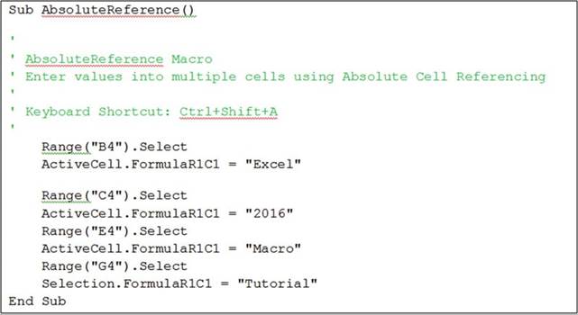
Figure17-16.CodeforAbsoluteReferencemacro
You can make changes to the code to alter the way the macro works. Notice that the code is placed between Sub
and End Sub statements. The Sub statement is given the name you assigned to the macro. After the Sub
statement comes several lines that start with a single quote. These lines appear in green. These are comment
lines. These lines are ignored when running the macro. They only appear as an aid to help you remember
important facts about the macro.
Next comes the code statements that make the macro perform
its steps. Notice
that cell addresses are placed in Range statements. These statements select
these exact cells.
That is why when you ran the macro the data was entered into the exact
same cells as they were originally entered.
659
CHAPTER 17 ■ AUTOMATING TASK WITH MACROS
We will change the code so that the first
cell used is no longer cell B4 but whatever cell you are in when you start the
macro.
4.
Change the statement Range("B4").Select to ActiveCell.Select
5.
Change the statement Range("C4").Select to ActiveCell.Offset(0, 1).Select
The range C4 is one column over from cell B4; therefore, we need our code to reflect the move one column over
from the active cell.
We can do this using
the Offset method.
The Offset method
uses two values.
The first value
is the row. The second
value is the column. We want all of our data to appear on the same row so we don�t
want to change
the row from the active
cell. Therefore, we use a 0 for the row to keep it where
it is and we use a 1 to move over one column.
6.
Change the statement Range("E4").Select to ActiveCell.Offset(0, 2).Select
The range E4 is two columns over from cell
C4. We also want our code to move
two columns over from the active
cell. Therefore, we use 2 for the column value of the Offset method.
7.
Change the statement Range("G4").Select to ActiveCell.Offset(0, 2).Select
The range G4 is two columns over from cell E4. We also want our code to move two columns
over from the active cell. Therefore, we use 2 for the column value of the Offset method. Your code should
look like the following:
ActiveCell.Select
ActiveCell.FormulaR1C1 = "Excel" ActiveCell.Offset(0, 1).Select
ActiveCell.FormulaR1C1 = "2016" ActiveCell.Offset(0, 2).Select
ActiveCell.FormulaR1C1 = "Macro" ActiveCell.Offset(0, 2).Select
Selection.FormulaR1C1 = "Tutorial"
Now that you have finished
editing the code you can return to the worksheet
to try it out. You can return to the worksheet by clicking the Excel
 �button on the toolbar or you can press Alt + F11. Pressing Alt + F11 lets you toggle back and
forth between the VBA Editor and the worksheet.
�button on the toolbar or you can press Alt + F11. Pressing Alt + F11 lets you toggle back and
forth between the VBA Editor and the worksheet.
8.
Press Alt + F11.
9.
Click inside cell C6. Press the
shortcut you created: Ctrl + Shift + A.
Try running the macro in different rows starting in different columns. The pattern should remain the same.
This exercise
solved the problem that you
observed in Exercise 17-2. You could
have, of
course, avoided the problem by
creating a Relative Cell Address
macro rather
than an
Absolute Cell Address macro.
660
Creating Macros
from Code
CHAPTER 17 ■ AUTOMATING TASK WITH MACROS
A macro doesn�t have to be
recorded and then played back. Macros can be manually coded into procedures in the Visual Basic Editor�s
code
window. You can still assign shortcut keys and a description to manually coded macros as well as assigning
them
to objects such as buttons, clip art, images, shapes, and so on.
A procedure is stored within a module. A module can contain many procedures. Macros are automatically
stored in numbered modules. The first macro you create will be stored in Module1. Each macro you
create thereafter will also be stored there until you close your workbook. When you reopen the workbook and
create a new macro it will be stored in Module2. Whenever you close and reopen the
workbook any new macros
that you create
will be stored
in a new module with the name assigned to the next number in the sequence.
Sometimes just a simple macro can greatly
improve the functionality of a worksheet. In this practice
we will create
the time line in Figure
17-17. Entering text at angle
saves space and looks good,
but you have to bend your head to view it. Wouldn�t
it be nice if you could view that vertical
text in a large cell in a horizontal format
without altering the current layout
of your data?
Well that is the functionality we are going
to add to the timeline. This practice program
will allow a user to click one of the cells that contains text displayed at an angle
and then either
use a shortcut key or click a button to copy the data to a cell that displays
the data in a horizontal format.
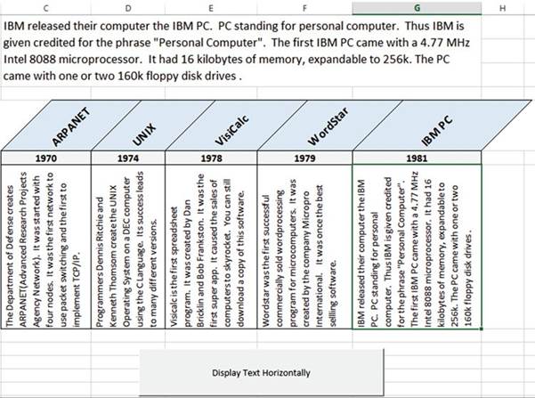
Figure17-17.Youwillcreatethistimeline
661
CHAPTER 17 ■ AUTOMATING TASK WITH MACROS
1.
Open the workbook Chapter 17.
2.
Click the Ribbon�s Developer tab. In
the Controls group click the Insert button.
3.
Click the Button
control in the Form Controls
area. Move the cursor below
the timeline and drag out a button
so that it is in the same location and size as shown in Figure 17-17.
4.
The Assign Macro button dialog
box appears. Fill in the fields as in
Figure 17-18:
a.
Change the Macro Name to
ConvertToHorizontal.
b.
Change the Macros in to This
Workbook.
c.
Click the New button.
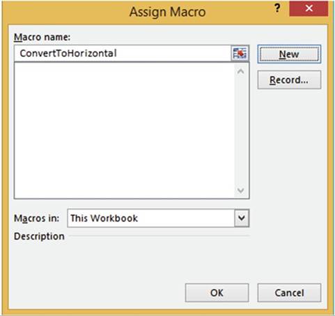
Figure17-18.ClicktheNewbuttonontheAssignMacrowindow
You are now in the VBA coding
area. The following code is displayed
in the Module code window.
Sub
ConvertToHorizontal() End Sub
5.
Place the following
code between the two Sub lines.
662
CHAPTER 17 ■ AUTOMATING TASK WITH MACROS
'Make the background
color white for the cell range C7:G7 Range("C7:G7").Interior.Color =
RGB(255, 255, 255)
'Make the background
color green for the selected cell ActiveCell.Interior.Color = RGB(110, 255,
170)
'Take the data from
the current cell and display in cell C1 Range("C1") = ActiveCell
6.
Press Alt + F11 to return to the worksheet.
7.
Click cell G7. Click the button you created.
The text
from cell G7 should appear in cell C1 in a horizontal format.
8.
Click cell C7. Click the button you created.
The text
from cell C7 should appear in cell C1 in a horizontal format.
9.
On the Developer
tab in the Code group click the Macros button.
Click the Options
button on the Macro dialog box. See Figure 17-19.
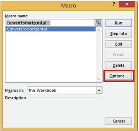
Figure17-19.SelectOptionsfromtheMacrodialogbox
10.
Complete the Macro Options dialog box shown in Figure 17-20:
a.
For the Shortcut key; hold down the Shift key and press T.
b.
For the Description, enter �Display text in horizontal format.�
c.
Click the OK button.
663
CHAPTER 17 ■ AUTOMATING TASK WITH MACROS
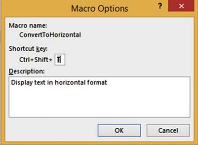
Figure17-20.EnterTfortheShortcutkey
11.
Click the Cancel button for the Macro window.
12.
Click one of the cells in the range C7:G7.
Press Ctrl + Shift + T. The ConvertToHorizontal macro runs and produces the timeline formatted like the one
shown previously in Figure 17-17.
Summary
If you find yourself
needing to perform the same steps over and over, then create a macro to save
yourself some time. Macros can be
played back by using shortcut keys. Macros can also be played by clicking
buttons or other objects that you
assign the macro to.
Macros that you want available to all of your workbooks, or to share with others, should be stored in the
Personal.xlsb workbook. This workbook
stays hidden until you click the Unhide button.
Macros can be
created using either relative addressing or absolute cell referencing. Absolute
cell referencing works okay when
you are creating a macro that affects a single cell, but if the macro affects multiple cells you will most
likely
want to use relative cell addressing.
Excel converts the macros that you create into Visual Basic for
Applications code. This code is editable. You don�t have to
create a macro to create VBA code. You can create your own VBA code from
scratch. After you have mastered learning VBA, you will find
yourself more often writing the code than letting Excel create it for
you.
664
Index
■
A
Absolute cell references, 257 AutoFill handle,
255�256
cell
address, 256
Account group, 218
Adding and removing worksheets available templates, 40�41
insert dialog box, 39�40
new sheet button, 39 Alignment group
buttons, 119
Home
Tab, 118 indentation of text, 123
merging and unmerging cells, 121, 123
rotating text, 124�125
Shrink to fit, 120
text wrapping, 119
vertical and horizontal, 123
worksheet, students
information, 125�128 American
Standard Code of Information
Interchange (ASCII), 53 AND function
logical conditions, 286 nesting, IF
function, 288�291 return FALSE, 286
syntax, 286
tool tip, 288
Arrange Windows dialog box, 388
Audio file, 631�633
AutoCalculate Tools feature
AutoSum feature
AutoSum
button, 229�230
Ctrl key, 231
handling blank cells, 232 location, 229
summing, rows and columns,
231 Average, Count Numbers, Max(imum),
Min(imum) AutoFill Handle, 235
auto functions, 234
cell styles,
236
more button,
236
thick outside
border, 237 wrap text, 233
wrong range, 235
AutoComplete feature,
70�71, 73 AutoCorrect feature
Add Items, 66
AutoCorrect dialog box, 67�68 caps lock key, 68
delete items, 70 AutoFill feature
Autofill Options
button, 76�77, 79�80
custom list, 78
duplicate cells creation, 73�74 option Copy Cells, 81
pattern, 75,
79
series of values, 74�75
■
B
Backstage
account group, 218 Info group
check for issues, 180�183,
185
information, 174�175
properties pane, 175�177
protect workbook
options, 178�180 Navigation pane and descriptions, 173�174 New group,
templates, 185�188
Open group,
workbook number of workbooks, 191 quickly access,
number of
workbooks, 191�192
recent list, 188�190 printgroup (see Printing options)
Save and Save Asgroups
(see Save and Save As groups)
Sharegroup (see Sharing workbooks)
665
■
INDEX
Bing Maps
Insert tab, 634
locations, 635�637,
640
move, resize
and delete, 640�641
panning and zooming,
639
pie charts,
637�638
street-level map, 640
visual representation, 634
■
C
Cell comments adding, 82�83
default name, 83
delete, 85
edit, 85
editing and deleting, 84 printing, 84�86
red triangle,
82
Ribbon�s Comments
group, 82 Show Ink button,
82
view, 83, 85
Cell reference, 19
Character code, 53 Charts
changing chart types, 459�464
Column chart, 448
combination (see
Combination chart) creation and modification
border, 452
Chart Elements
drop-down box, 449�450
Cool Slant, 452
2D Clustered bar chart,
448 effects, 452
Fill & Line paint
bucket, 451 Format Selection pane, 450, 455 Game Sales tab, 449
Gradient fill, 454
Horizontal (Category) Axis, 450
Light Gradient � Accent 2, 455
Pattern Fill options, 454
Plot Area, 450
Shadow options,
453
size, 449
Text options,
453
Title Options
menu, 450 hierarchicalcharts (see Hierarchical charts)
Insert Chart dialog box, 446�447 piecharts (see Pie
charts)
quick layouts, 459 Ribbon�s Insert tab, 445 series color, 464
sparklines (see Sparklines) styles
Bar charts,
456
changing, 457�458
Chart Elements
button, 457 Data Labels, 457
Data Table,
457
More button, 456 Clearing contents, cell, 64�65
Cloud Application, 621�622 Column widths
adjusting,
57, 60
changing, 57
checking, 56
dialog box, 57
exponential notation,
56
format button,
58
hidden text, 55
multiple columns,
58�59
resizing, 58
# signs, 56
text overflow,
next cell, 55 Combination chart
Bold button,
480
clustered column chart, 478 column and line chart, 477 creation, 477�480
Line with Markers, 479 title change,
480
Compatibility Checker, 184
Context-sensitive tabs,
9 Custom view
Add View, 170
create, 170
Custom Views dialog box, 169
delete, 171
Show, 171
■
D
Data
entry, multiple worksheets, 405�409 Data protection
cell-level, 340�341
Worksheet-level, 336�339 Data types
date and time data, 50 numeric
data, 49
text data, 49 Data validation
creation
circling invalid data, 317
custom restriction, 315�316 Error Alert message, 310�311 error message, 309
formula, Order ID, 307
Information Style Error
Alert, 314�315 Input Message tab, 307�308 instruction, 306
syntax, LEFT function, 306
list restriction, 312�314
666
■
INDEX
settings tab, 306
size of validation area, 317�318
warning style and time restriction, 311�312
Data Tools group, 304
dialog box, 304
options, 305 Date functions
NOW function, 295�296
serial number, date, 297�298
TODAY( ) function, 293�294
Date slicer,
567
Deleting columns
and rows, 139�140 Delimited text files
changing data, 515�518 comma-delimited text file, 504 connection, imported
file and
workbook, 514�515
connections, 512
Existing Connections dialog
box, 511 Existing Connections window, 511 external data, 508�510
header row, 504
Import Text File dialog
box, 512 refresh
all button, 513
Text Import
Wizard, 505�507 Dialog box launchers
format cells, 12 Document recovery
AutoRecover time interval, 196
Excel Options window, 194�195
Manage Workbook button, 200
recoverable unsaved
workbooks, 199 recovered files, 197�199
unsaved files,
200
■
E
Entering and correcting data AutoComplete feature,
70�71
AutoCorrect feature, 65�70 AutoFillfeature
(see AutoFill feature) clearing
contents, cell, 64�65 Columnwidths (see Column widths) Pick from
Drop-down List feature, 71�72 row
heights, 61�62
special character insertion, 51�54 typing
mistakes
cell to its original
value, 63�64 specific
characters, 63
Entering formulas arrow keys, 222
AutoCalculate Toolsfeature (see AutoCalculate Tools feature)
built-in
functions, 223�224
cell address corresponding cell color, 224 clicking the cells, 222
formula bar, 225
goods sold computation, 225
markup % computation, 225
math operations, 223
profit computation, 226
spreadsheet formulas, 223
typing, 222 Excel
cell reference, 19
creation, workbook, 8�9 current (active) cell,
19 description, 1
entering data, worksheet, 19�21
insert chart window, 24
navigation basics
components, workbook,
3
QAT (see
Quick access toolbar
(QAT))
ribbon (see
Ribbon)
save as option, 6�7 screen tips, 22
Smart Lookup,
24�26
starting window,
5
tell me what you want to do feature,
22�23
■
F, G
Fill Across Worksheets copy command, 385, 387 Fixed-width text files
import Data window, 521
Import Text File dialog box, 519
Text Import Wizard, 519�520
Flash Fill
data, worksheet, 358
description, 357
features, 359�361,
363
Home tab, 358�359
result of, 359
Format Painter,
copy formatting, 129�132
Formatting data
cell background color, 96�99 cell borders
Border Button,
103
Draw Borders Grid tool, 106
Draw Border tool, 102�105
Erase Borders, 109
Format Cells
Dialog Box, 106�108
options and tools,
102
types, 100�101
unchecking gridlines, 99
font color, 94�95 font group
bold, italics,
underline and double underline, 90
command buttons,
89�90 dialog box launcher, 93
font and size changing, 90�92
667
■
INDEX
Formatting numeric data, number group accounting and currency formats, 112 comma style, 114
decimal places,
114
default formats,
data types, 111 description, 110
exercise, 115�118
format cells dialog box, 114�115 monetary
values, 112�113
percent style, 113
Formula auditing
nested function, 327�330
tools, 322
tracing precedents and dependents, 322�325
Watch window, 325�327
Formula evaluation
circular reference, 320,
322 error value messages, 319 IFERROR function, 319�320
Formulas
absolute cell references, 257 alphabetic data,
256
AutoFill handle, 255, 258
cell addresses, 256
travel expense
report, 257�259 addition,
220
copying
additional records,
226
AutoFill Handle,
227
dragging, AutoFill
Handle, 227 Fill Handle, 226
relative cell referencing, 226 rows,
228
entering (see Entering formulas) formula bar, 221
math symbols, 219�220
mixed cellreferences (seeMixed cell referencing)
named constants creating, 249�250
named ranges
built-in functions, 251
changing name, 246�247
creation, 248
define Name, 246
Name Box, 246
removing, 247�248
scope, name, 252�254 size, Name Box, 247
named ranges and constants deleting, 242
editing, 241�242
Name
Manager, 241
naming constants, 240 naming ranges
characters, 238
defined Names group, 238�239
New Name dialog
box, 239 noncontiguous, 239�240
refers to text box, 239
scope drop-down box, 239
order of precedence, 263
row or column headings, range names, 242�244
viewing, 237
Freezing
Pane options,
165
rows and columns, 164 Functions
AND function,
286
categories, 265�266 construction
arguments, 267
IF function,
267
logical functions, 267
syntax, 267
datefunctions (see Date
functions) DAYS function, 300, 302
DAY, YEAR, and MONTH functions, 298�300
nested functions, 287
OR function, 286�287
summing cell values
cell address,
280
IF function,
283
Insert Function Option,
270�273 optional sum_range argument, 278 SUM function, 268�270, 272�273
SUMIFS Functions, 278�282
■
H
Hiding and unhiding rows and columns, 137�138
Hiding and unhiding worksheets, 42
Hiding columns and rows, 134 Hierarchical charts
Sunburst chart, 488
accent 5, 491
advantage, 487
3D effect,
493�494
dialog box launcher, 492 enlarge, 490�492
removing values, 488�489
selection, individual slice, 495
value, slice, 489
Treemap chart Banner, 482
Colorful group, 483
colors, rectangles, 483 labels and values,
484�485 picture or texture
fill, 487 See all Charts button,
481
668
■
INDEX
select Data Labels, 483�484
texture background, 486
triple-click, cookies
rectangle, 486 Hyperlinks
concatenation, 356�357
create, Excel workbook, 355�356
description, 343
file
Address box, 350
Browse for File button,
351 create text, notepad, 349
Insert Hyperlink dialog box, 350 message,
353
select All Files, 351�352
FlashFill (see Flash Fill)
Insert Hyperlink Window, 344
location, workbook, 354
status bar
Average, Count,
Numerical Count, Minimum,
Maximum and Sum, 367
Caps Lock, Num Lock, 366, 370
Cell Mode, 366, 370
computations, 369
data, worksheet, 368
End Mode, 367
Fixed
Decimal mode, 367 Flash Fill, 366
macro recording, 367
options, 364�365
Overtype Mode, 367, 370
Page Number, 367
Scroll Lock, 366, 370
Selection
Mode, 367, 369�370
View Shortcuts, 367
Zoom and Zoom Slider,
368, 371 web pages
Apress Corporation, 346
AutoFormat As You Type tab, 345�346
context menu, 347
e-mail address,
347
Screen Tips, 348
URL address,
345
■
I, J, K
IF function
AutoFill Handle,
285
Create Names from Selection
dialog box, 284 formatting the range, 285
overtime pay formula, 283 syntax, 282
Importing data access database
Import Data dialog box, 523 multiple
tables, 522
Select data source, 522 select table/query, 523
updating data, 523
view data, 523
Get
External Data group,
503 query feature
calculated Column creation, 532�534
choosing fields, 530
closing and loading, 538�539
Edit button, 529
fields, choosing of, 529 filter, 530
Get & Transform group, 527 merging
queries, 534�537 moving column heads, 537 naming tables, 529
select
multiple items, 528�529
Undoing and Redoing Query Steps, 531�532 web address, URL text box, 527
text files
delimited (see Delimited text files) fixed-width, 518�521
web site
imported data, 526
New
Web Query dialog
box, 524�525 selecting tables, 525
Insert Copied Cells, 400�403
Insert Cut Cells, 403�404
Inserting and deleting cells, 140�142
Inserting columns and rows, 139
■
L
Lotus
1-2-3 Spreadsheet program,
2
■
M
Macros
absolute cell references, 646�648
assign Macro window, 662
description, 643
developer tab, 662
macro-enabled
workbooks, 648�649
module, 661
options, 663�664
Personal Workbook, VBA code,
658�660 Quick Access
Toolbar
Customize, 652�653
Developer tab, 656�657 Form Controls
and and
ActiveX Controls, 657�658
shapes, 654�655
View tab, 656 recording
create, 644�646
669
■
INDEX
Macros (cont.)
locations, 643
Macro Recorder,
643
play back,
646
Record Macro
dialog box, 644 Start Recording button, 644
relative cell references, 650�651
time line, 661
Microsoft Office Clipboard, 404�405 Microsoft Office Themes, 444
Mini-toolbars and context menu,
132�133 Mixed cell referencing
description, 259
formulas, 262
multiplication table
creation, 260�262 Multimedia
audio sounds,
631�633 BingMaps (see Bing
Maps) description, 591
pictures
adjustments, 595�596
Bing Image Search text box, 592 border, 598
Format tab, 594
glow effect, 599
Insert Picture window, 592
Insert tab�s
Illustrations group, 591, 593
pencil sketch and photocopy, 596�597 Picture Styles Gallery, 597�598
Pilot picture,
593 sharpness, brightness and
contrast, 594�595
screenshot, 599�602 shapes
changing and moving, object,
622�623 flowchart, 610�618
gallery, 609
grouping and ungrouping, 618�622
image conversion, 624
SmartArt (see SmartArt) video
file, 633
WordArt (seeWordArt)
■
N
Naming worksheets, 39
■
O
Order of precedence, 263 OR function
logical conditions, 287
nesting, IF function, 291�292 returns TRUE, 287
syntax, 286
■
P
Panes
horizontal and vertical scroll
bars, 164 size, 163
split bars, 163�164
split
Window button, 162 vertical, 162
Paste button gallery
AutoFit, column width, 381 copied data, 382
formatting, cell contents, 383
options, 379�384, 389�390
tooltip, 379 Paste Special
dialog box, 391
gallery, 390�391
operation options, 392 perform
calculations
Add operation, 395�397
Multiply operation, 398�399 Skip Blanks option,
400
transpose rows and columns,
393�395 use, 393
Pick from Drop-down List feature, 72 access, 71
Pie charts,
469
creation, 465�468
description, 465
labels, 465 pie of
to Bar of Pie, 476 Data Callout, 471 2-D Pie area, 470
Series Options button, 471�472 Split
Series by, 472�473 worksheet tab, 469
Quick
Analysis button, 466 Split Series
By
custom, 474�476
Percentage value, 474
value, 473
Style 10 applied, 467
Title Options,
468
variations, 446 PivotChart and PivotTable
category and product fields,
572 clear, 579
Clustered Column chart, 574 delete, 579
existing worksheet, Location text box,
569�570 filter buttons, 570�571
Format As Table dialog box, 569 Insert Chart dialog box, 573
multiple tables, source data, 575�578 product data, 571�572
670
■
INDEX
PivotTables
benefit, 541
collapse and expand, categories, 545�546
data filtering, 547�548
data source
location, 552�553
data,
Work & Leisure
Company, 542 dialog
box, 542
existing Worksheet, 542
field order, 549
field removal, 550
fields list, 543�545 handling
dates and times
adding records and refreshing, 565�568
creating table, 556�561
data conversion, 555
grouping and ungrouping fields,
562�565 inventory data, 555
spreadsheet, 555
table
name, 556
recommended, 554
relationaldatabases (see Relational database, PivotTables)
Sum
function, 550�551 viewing
field Values, 546
Printing
additional cells, print area, 158 creation, Print area, 157 Ignore Print Area, 160
Paste
Special, 160�161 removing, Print Area, 158
Printing options collating, 208
orientation, 209
page margins, 210�211
paper size, 209
Print Active Sheets, 207
Print Entire Workbook, 208
printer selection, 206
scaling options, 211�213
settings, 205�206 Proofreading cell values, 331�333
■
Q
QAT. See Quick access toolbar (QAT)
Quick access toolbar (QAT), 331�332, 15
command buttons,
18
customize quick access toolbar, 15
touch/mouse mode button, 16�17
■
R
Relational database,
PivotTables areas, 586�587
Create PivotTable dialog box, 583�584
customer table, 579�580
fields, 584�587
Manage Relationships dialog box, 582�583
master and detail tables, 579, 581
orders table, 579�580
results, 588
Reordering and copying worksheets, 43 Ribbon
contextual tabs, 9�10
dialog box launchers, 11�12 Maximize button, 11
options, 13
resizing, 10�11
Restore Down button, 11 shortcuts
home tab commands, 14
merge & center category, 14
merge & center option, 14
tabs and QAT, 14
tabs, 9
Row heights,
61�62
■
S
Save and Save As groups AutoRecover feature, 192
documentrecovery (see
Document recovery) file
types, 193
Inventory_063011, 193
OneDrive, 194
path,
drive and folders,
194 protections
Backstage
messages, 205
General Options dialog box, 201�202
passwords, 202�204
tools options,
201
random access
memory (RAM), 192 Screenshot, 599�602
Screen tips, 22, 26 Selecting cells,
worksheets
cell
reference, name box, 35�37
go to feature, 37�38
keyboard
area, 34�35
column, 34
current cell to last cell, 35 entire block, 35
entire worksheet, 35
multiple columns,
34
multiple rows, 34
rows, 34
worksheet ranges, 33 mouse
adjacent cells, 32�33
cells, 33
671
■
INDEX
Selecting cells, worksheets (cont.) nonadjacent cells, 33
rows or rolumns, 31�32 worksheet ranges,
31
Sharing workbooks
Files using E-mail, 217�218
Online with OneDrive, 214�216
SmartArt
definition, 625
organizational chart
arrow button, 626 color, Shape Fill, 630 create, 625�626
gridlines, 628, 630
image VPofSales, 630 Name and Title, 627�629
text block, 626�627
Sparklines
clearing, 500
creation, 496�499
data location and location,
500�501 description, 495
grouping, 500
negative values,
496
Ribbon�s Sparklines group, 496 ungrouping, 499
wins and losses, 496 Special characters insertion
categories, symbols,
53
Character code,
53
symbol button,
52 symbol dialog box, 52
Spell
checking, 333�334 Spreadsheets
Excel (see Excel)
Lotus 1-2-3
Spreadsheet program, 2
VisiCalc, 2 SUM function
additional argument, 269
arguments,
268, 269
constants, 270
syntax, 268 SUMIFS function
argument descriptions, 279
bank deposits summing, 279 breaking, formula, 281 handling empty cells, 281�282
required arguments, 276�277
syntax, 276,
278
Synchronous scrolling, 165�168
■
T
Tables
adding to Excel
automatic
expansion, 414�415
create tables and apply filters, 415�422 cell styles, 429�432
conditional formatting applying to table,
441�444 clear rules,
434
data, orders
tab, 432
edit, delete and create new rules,
438�439 highlight, data bars, 435�436
highlight duplicate/unique values, 436
highlight specified text, 438
highlight values between other values, 437 highlight values
greater than another
values, 437 top/bottom rules, 433
creating and formatting, 411�413
description, 411
filtering data, slicers, 422�424 sort
and filter, 413�414 themes, 424�429
Thesaurus, 334�335
Time slicer,
568
Transferring and duplicating data description, 373
Fill Across
Worksheets copy command, 385, 387
move and copy cell data
cut
and copy buttons,
376 cut and paste, 377
drag-and-drop method, 374�376
duplicate cell contents, 378 keyboard shortcuts, 377
pasteoptions
(see Paste button gallery)
Typing mistakes
restoring cell to original
value, 63�64 specific
characters, 63
■
U
Unhide Column A or Row 1, 136�137 Unhiding
columns and rows, 135
■
V
Video file, 633 Viewing
page break preview
horizontal page break line, 147�148
inserting page break, 149
location, page breaks, 149 Print
Preview pane, 149 remove page break, 149 reset page breaks, 149
Row
and Column Headers,
150�151 types, 146
vertical page break line, 147�148
672
■
INDEX
Page Layout view
header and footers, 152�154
header sections, 152
Print Worksheet, 154
Remove Whitespace, 155�156
Scale and Alignment of your Headers
and Footers, 154�155
Show Options
Off and On, 156
VisiCalc, 2
■
W, X, Y, Z
Website, importing data
Get External
Data group, 524
New
Web Query dialog box, 524�525
selecting tables, 525
storing,
imported data, 526 WordArt
circle within the text, 608�609 definition, 603
Font Type, 603
Insert tab, 603
Styles group,
604
Text Effects, 605, 607
text fill options, 604
text
options dialog bo x, 605�606
texture, 604
Worksheets
adding and removing, 39�41
hiding and unhiding, 42 moving between
cells, keyboard
arrow keys, 30
entering values,
28
file tab, 29
pagedown key, 30 page up key, 30 saving,
29
shift+ tab key, 30
shortcut movement keys, 28 tab key, 29
naming, 39
reordering and copying, 43 selecting
cells
cell
reference, name box, 35�37
keyboard, 33�35
mouse, 31�33
select multiple, 42
tab
buttons, moving, 44�48
tab color, 41�42
673